Neil A. Duffie - Control Theory Applications for Dynamic Production Systems

Variables in discrete-time models have a value only at discrete instants in time separated by a fixed time interval T . While many physical variables in production systems are fundamentally continuous, they often are sampled, calculated, or changed periodically. Examples include work in progress (WIP) measured manually or automatically at the beginning of each day, mean lead time calculated at the end of each month, and production capacity adjusted at the beginning of each week. Discrete-time modeling results in difference and algebraic equations that describe input–output relationships and represent the behavior of a production system at times kT where k is an integer.

The production work system illustrated in Figure 2.6 can be represented by a discrete-time model that predicts work in progress (WIP) at instants in time separated by fixed period T . This period could, for example, be one week ( T = 7 days), one day ( T = 1 day), one shift ( T = 1/3 day) or one hour ( T = 1/24 day). The modeled values of work in progress then are ww ( kT ) hours. If it is assumed that work input rate ri ( t ) hours/day, nominal capacity rp ( t ) hours/day, and capacity disturbances rd ( t ) hours/day are constant (or nearly constant) over each period kT ≤ t < ( k + 1) T days, the work output rate at time kT days then is

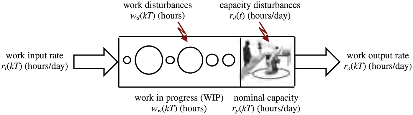
Figure 2.6 Discrete variables in a discrete-time model of a production work system.

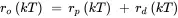
and the WIP is

This discrete-time model only represents the values of WIP ww ( kT ) at instants in time separated by period T ; values between these instants are not represented. When the inputs are constant during period kT ≤ t < ( k + 1) T , it is clear from the model obtained in Example 2.1 that ww ( t ) increases or decreases at a constant rate over that period; however, this information is not contained in the discrete-time model.

The dynamic behavior represented by this discrete-time model is illustrated in Figure 2.2 for a case where T = 1 day and there is a capacity disturbance rd ( kT ) of –10 hours/day that starts at time kT = 0 and lasts until kT = 3 days. The initial WIP is ww ( kT ) = 30 hours for kT ≤ 0 days. The rate of work input is the same as the nominal production capacity, ri ( kT ) = rp ( kT ), and there are no WIP disturbances: wd ( kT ) = 0. In this case, the difference equation for WIP can be written as

The response of WIP to the capacity disturbance, with the other inputs constant, is shown in Figure 2.7 and calculated recursively in Program 2.2 using the this difference equation. In Figure 2.7, the responses are denoted by the discrete values at times kT as well as by a staircase plot. The latter is used by convention to indicate that no information is present in the discrete-time model regarding the WIP between the instants in time separated by period T . 4

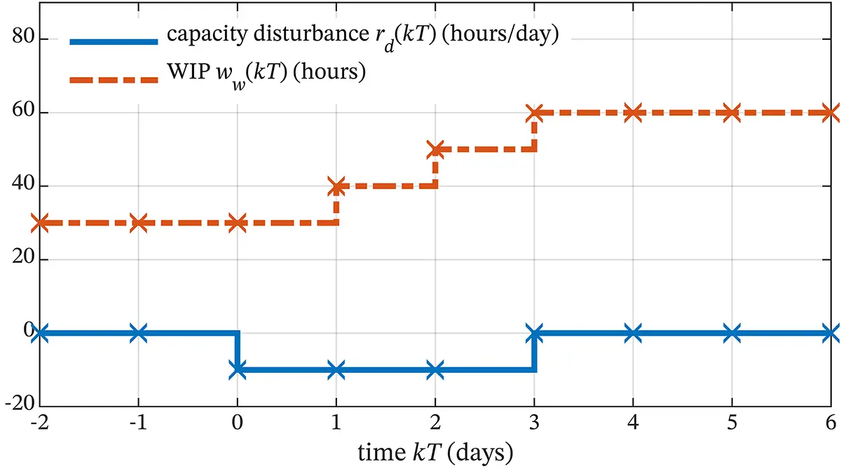
Figure 2.7 Response of WIP to a 3-day capacity disturbance; each discrete value is denoted with an X.

T=1; % discrete period (days) kT=[-2,-1,0,1,2,3,4,5,6]; % times kT (days) rd=[0,0,-10,-10,-10,0,0,0,0]; % capacity disturbance at times kT (hours/day) ww(1)=30; % initial WIP at time kT=-2 days (hours) for k=-2:5 % instants in time kT between kT=-2 and kT=5 days ww(k+4)=ww(k+3)-T*rd(k+3); % next WIP end stairs(kT,rd); hold on % disturbance and WIP vs kT - Figure 2.7 stairs(kT,ww); hold off xlabel('time kT [days]') legend ('capacity disturbance r_d(t) (hours/day)','WIP w_w(t) (hours)')

The decision-making component shown in Figure 2.8 is used to calculate periodic adjustments that increase or decrease the lead time used to plan operations in a production system. Lateness of order completion can negatively affect production operations and customer satisfaction, and it is common practice to increase planned lead times when the trend is to miss deadlines. On the other hand, planned lead times can be decreased when the trend is to complete orders early; this can be a competitive advantage because earlier due dates can be promised when customers are placing or considering placing orders.

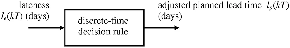
Figure 2.8 Discrete-time decision-making component for adjusting planned lead time in a production system as a function of lateness of order completion.

An example of a discrete-time decision rule that could be used periodically to adjust planned lead time is

where lp ( kT ) days is the planned lead time, ∆ lp ( kT ) days is the change in planned lead time, le ( kT ) days is a measure of lateness that could be obtained statistically from recent order due date and completion time data, and Kl weeks is a decision-making parameter that needs to be designed to obtain favorable dynamic behavior of the production system into which the decision-making component is incorporated. T weeks is the period between adjustments. This decision rule both increases planned lead time when orders are late and also increases planned lead time when lateness is increasing; the contribution of the latter is governed by the choice of parameter Kl .

The dynamic behavior of the component is illustrated in Figure 2.9b for the case shown in Figure 2.9a where lateness le ( kT ) increases to 8 days over a period of 6 weeks. The response of change in planned lead time to this increase in lateness is shown in Figure 2.9b for Kl = 2 weeks and Kl = 4 weeks. The period between adjustments is T = 1 week. The response was calculated recursively using the above difference equation in a manner similar to that shown in Program 2.2. As expected, the larger value of Kl results in larger adjustments when lateness is increasing, a stronger response to this trend in lateness.