Neil A. Duffie - Control Theory Applications for Dynamic Production Systems

(2.4)

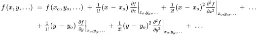
Over some range of ( x – x o), ( y – yo ), … higher-order terms can be neglected and a linear model is a sufficiently good approximation of the nonlinear model in the vicinity of the operating point:

(2.5)

where

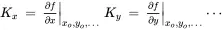(2.6)

In the case where the production work system illustrated in Figure 2.15 has variable work in progress (WIP) w ( t ) hours and variable production capacity r ( t ) hours/day, the lead time is

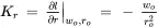
For work in progress operating point wo and capacity operating point ro , an approximating linear function for lead time in the vicinity of operating point wo , ro , can be obtained using Equations 2.5and 2.6:

where

In practice, variables in models of production systems may have a limited range of values. Maximum values of variables such as work in progress and production capacity cannot be exceeded, and these variables cannot have negative values. In many cases, operating conditions where limits have been reached may not be of primary interest when analyzing and designing the dynamic behavior of production systems. On the other hand, models can be developed that represent important combinations of operating conditions, each of which represents dynamic behavior under those specific conditions. A set of piecewise linear approximations then can be used to represent non-linear relationships between variables.

The relationship between work in progress (WIP) and actual capacity shown in Figure 2.17 is another example of nonlinear behavior. When WIP w ( t ) is relatively low in a production work system such as that shown in Figure 2.15, production capacity may not be fully utilized and actual capacity can be less than full capacity because of the work content of individual orders and the timing of arriving orders. Conversely, when WIP is relatively high, work is nearly always waiting and the work system is nearly fully utilized. The actual capacity ra ( t ) of the work system therefore may depend on both its full capacity rf and the work in progress w ( t ).

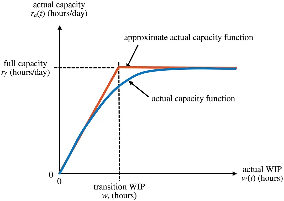
Figure 2.17 Actual production capacity function and a piecewise linear approximation.

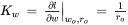
As shown in Figure 2.17, the actual capacity function can be approximated in a piecewise manner by two segments, delineated by a WIP transition point wt hours, where for w ( t ) ≥ wt

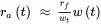
and for w ( t ) < wt

The examples that were presented in this chapter illustrate some of the ways that models can be developed for production systems and components. Production systems often have many components, and dynamic models of these components need to be obtained individually using physical analysis or experimental data. Then they can be combined if desired to obtain a model of the dynamic behavior of an entire production system. In Chapter 3, transformation methods will be introduced that allow algebraic equations to be substituted for the linear differential and difference equations that describe the dynamic behavior of components in a production system. These transformations make combining models of components relatively easy and they are compatible with the many analysis and design tools that are implemented in control system engineering software. As also described in Chapter 3, transformed models of production system components can be assembled into block diagrams that graphically represent the input–output relationships between components in production systems, aiding in identifying, understanding, and designing the dynamic behavior of production systems.

1 1 The term “discrete-time” differentiates this type of model from discrete-event simulation models.

2 2 Here and in subsequent examples, well-known solutions for the differential equations obtained are not derived. The tools of control system engineering that are presented in subsequent chapters generally make it unnecessary in practice for production engineers to find such solutions.

3 3 It often is convenient to use relative change as a variable in dynamic models of the components of production systems.

4 4 Henceforth, staircase plots will be presented without explicitly denoting discrete values at times kT.

5 5 The reader is referred to the Bibliography and many other publications on nonlinear dynamics and nonlinear control theory for other approaches to modeling nonlinear behavior.

6 6 Other options include choosing to regulate a variable other than lead time (work in progress, due date deviation, etc.) and designing non-linear decision rules.

Текст предоставлен ООО «ЛитРес».

Прочитайте эту книгу целиком, купив полную легальную версию на ЛитРес.

Безопасно оплатить книгу можно банковской картой Visa, MasterCard, Maestro, со счета мобильного телефона, с платежного терминала, в салоне МТС или Связной, через PayPal, WebMoney, Яндекс.Деньги, QIWI Кошелек, бонусными картами или другим удобным Вам способом.