Neil A. Duffie - Control Theory Applications for Dynamic Production Systems

The model obtained is highly dependent on the physical and logistical nature of the production system and the components being modeled. The utility of the model is highly dependent on the nature of the analyses that subsequently will be performed and the decision-making components that are to be designed as a result. For this reason, past experience in modeling, analysis and design plays a significant role in anticipating the model that is required. Furthermore, models usually need to be modified during subsequent steps of analysis and design: additional features may need to be added, additional simplifications may need to be made, and fidelity may need to be improved. Additionally, the nature of the decisions that are made in production systems, as well as the structure of the information and communication that is required to support decision-making may change as the result of understanding gained during analysis and design; this can require further model modification.

Variables in continuous-time models have a value at all instants in time. Many physical variables in production systems are continuous variables even though they may change abruptly. Examples include work in progress (WIP), lead time, demand, and rush orders. Continuous-time modeling results in differential and algebraic equations that describe input–output relationships at all instants in time t . Although the specific output function of time that results from a specific input function of time often is of interest, the goal is to obtain models that are valid for any input function of time or at least a broad range of input functions of time because the operating conditions for production systems and their components can be varying and unpredictable.

For the production work system illustrated in Figure 2.1 it is desired to obtain a continuous-time model that predicts work in progress (WIP) ww ( t ) hours as a function of the rate of work input to the work system ri ( t ) hours/day, the nominal production capacity rp ( t ) hours/day, WIP disturbances wd ( t ) hours and capacity disturbances rd ( t ) hours/day. WIP disturbances can be positive or negative due to rush orders and order cancellations, while capacity disturbances usually are negative because of equipment failures or worker absences. Units of hours of work are chosen rather than orders or items, and units of time are days.

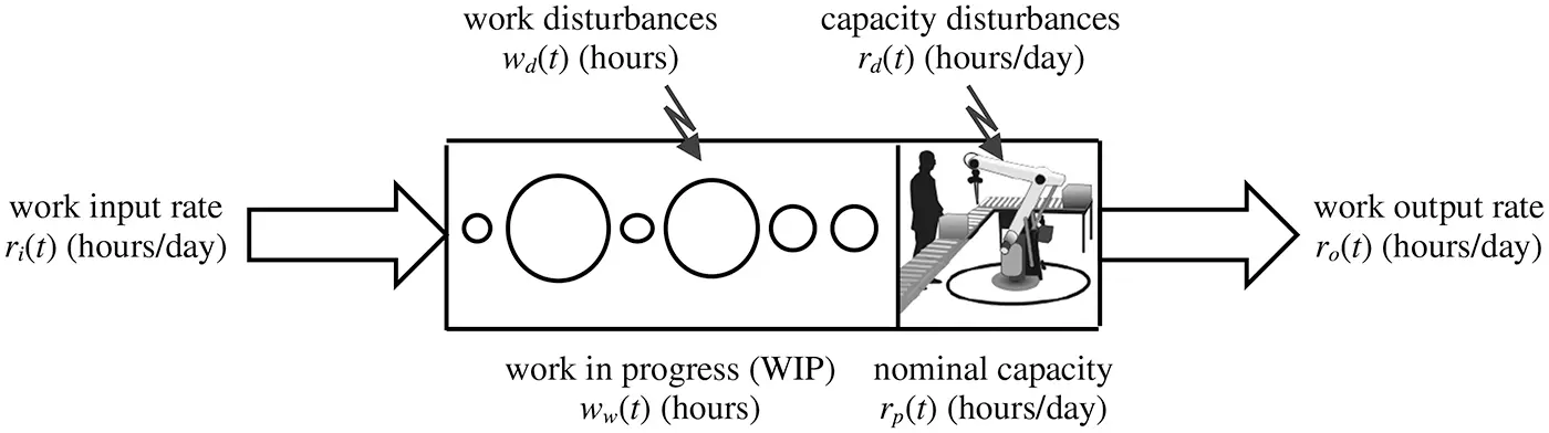
Figure 2.1 Continuous variables in a continuous-time model of a production work system.

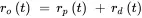
The rate of work output by the production system ro ( t ) hours/day is

The WIP is

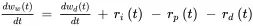
where ww (0) hours is the initial WIP. Integration often is an element of models of production systems and their components. The corresponding differential equation is

The dynamic behavior represented by this continuous-time model is illustrated in Figure 2.2 for a case where there is a capacity disturbance rd ( t ) of –10 hours/day that starts at time t = 0 and lasts until t = 3 days. The initial WIP is ww ( t ) = 30 hours for t ≤ 0 days. The rate of work input is the same as the nominal production capacity, ri ( t ) = rp ( t ) hours/day, and there are no WIP disturbances: wd ( t ) = 0 hours. The response of WIP to the capacity disturbance is shown in Figure 2.2 and is calculated using Program 2.1 for 0 ≤ t ≤ 3 days using the known solution 2

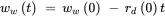
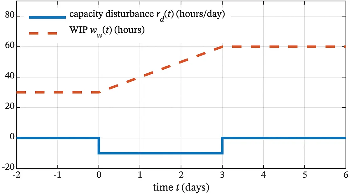
Figure 2.2 Response of WIP to 3-day capacity disturbance.

This model represents the production work system using the concept of work flows rather than representing the processing of individual orders. Numerous aspects of real work system operation are not represented such as setup times, operator skills and experience, reduction in actual capacity due to idle times when the work in progress is low, and physical limits on variables. Also, WIP cannot be negative and often cannot be greater than some maximum due to buffer size. Capacity cannot be negative and cannot be greater than some maximum that is determined by physical characteristics such as the number of workers, number of shifts, available equipment, and available product components or raw materials.

ww0=30; % initial WIP (hours) rd0=-10; % capacity disturbance (hours/day) t(1)=-2; rd(1)=0; ww(1)=ww0; % initial values t(2)=0; rd(2)=rd0; ww(2)=ww(1); % disturbance starts t(3)=3; rd(3)=0; ww(3)=ww(2)-3*rd0; % solution of differential equation t(4)=6; rd(4)=0; ww(4)=ww(3); % disturbance ends stairs(t,rd); hold on % plot disturbance and WIP vs time - Figure 2.2 plot(t,ww); hold off xlabel('time t (days)') legend ('capacity disturbance r_d(t) (hours/day)','WIP w_w(t) (hours)')

A continuous-time model is needed for the production system illustrated in Figure 2.3 that would facilitate design of an order release rate adjustment decision rule that tends to maintain backlog at a planned level. This type of decision-making can be referred to as backlog regulation, and it could operate manually or automatically. There are fluctuations in order input rate and disturbances in the form of rush orders and canceled orders that must be responded to by adjusting the order release rate in a manner that tends to eliminate deviations of actual backlog from planned backlog.

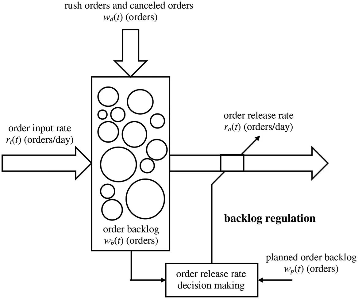
Figure 2.3 Backlog regulation in the presence of rush orders and canceled orders.

There are two main components: accumulation of orders in the backlog, and order release rate decision-making. The differential equation that describes backlog is similar to that developed in Example 2.1:

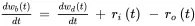
where wb ( t ) orders is the order backlog, wd ( t ) orders represents disturbances such as rush orders and order cancelations, ri ( t ) orders/day is the order input rate, and ro ( t ) orders/day is the order release rate.