Neil A. Duffie - Control Theory Applications for Dynamic Production Systems

The portion of production capacity provided by permanent workers is

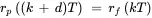
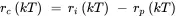
where dT days is the delay in implementing permanent worker capacity adjustments. Hence, the portions of fluctuating order input that are addressed by permanent worker capacity rp ( kT ) orders/day and cross-trained capacity rc ( kT ) orders/day are

A component behaves in a linear manner if input x 1produces output y 1, input x 2produces output y 2, and input x 1+ x 2produces output y 1+ y 2. The following are examples of linear relationships:

The following are examples of nonlinear relationships:

In reality, most production system components have nonlinear behavior, but often the extent of this nonlinearity is insignificant and can be ignored, with care, when a model is formulated. On the other hand, behavior that is significantly nonlinear often can be modeled in a simpler but sufficiently accurate manner using approximate linear models obtained using approaches such as those described in the following subsections. 5

A nonlinear function f ( x ) of one variable x can be expanded into an infinite sum of terms of that function’s derivatives evaluated at operating point x o :

(2.1)

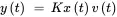
xo is the operating point about which the expansion made. Over some range of ( x – xo ) higher-order terms can be neglected, and the following linear model in the vicinity of the operating point is a sufficiently good approximation of the function:

(2.2)

where

(2.3)

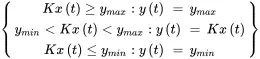
Such an approximation is illustrated in Figure 2.14.

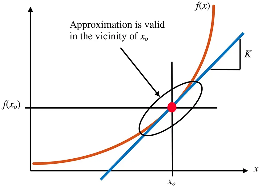
Figure 2.14 Linear approximation of function f ( x ) at operating point xo.

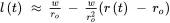
A production work system such as that illustrated in Figure 2.15 has constant work in progress (WIP) w hours and variable production capacity r ( t ) hours/day. The lead time l ( t ) hours then is approximately

Figure 2.15 Production work system with variable capacity.

The relationship between lead time and capacity is nonlinear; however, a linear approximation of this relationship in the vicinity of operating point ro can be obtained using Equations 2.2and 2.3:

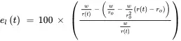
The percent error in lead time calculated using the linear approximation due to deviation of actual capacity r ( t ) from the chosen capacity operating point ro is shown in Figure 2.16 and calculated using

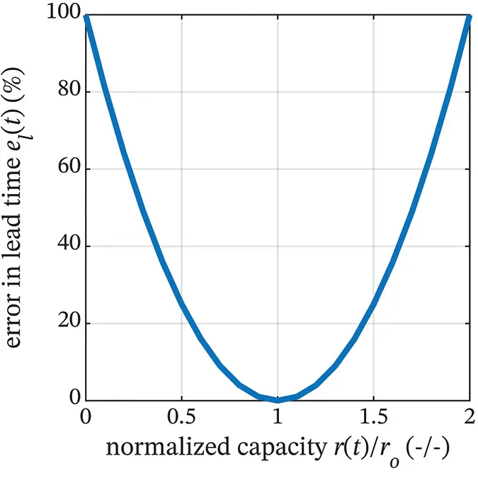
Figure 2.16 Percent error in lead time due to deviation of actual capacity from capacity operating point chosen for linear approximation.

Clearly, capacity should not deviate significantly from the operating point if this approximation is used in a model. If, for example, lead time is to be regulated by adjusting capacity, capacity might vary significantly from the operating point that was used to design lead-time regulation decision rules. An option 6in this case could be to

calculate the parameters for a linearized model for each of several capacity operating points

design lead time regulation decision rules for each operating point using the model for that operating point

switch between decision rules as operating conditions vary.

A nonlinear function f ( x,y,… ) of several variables x , y , … can be expanded into an infinite sum of terms of that function’s derivatives evaluated at operating point xo , yo , …: