Ray Kurzweil - How to Create a Mind - The Secret of Human Thought Revealed

We captured speech as a waveform, which we then converted into multiple frequency bands (perceived as pitches) using a bank of frequency filters. The result of this transformation could be visualized and was called a spectrogram (see page 136).

The filter bank is copying what the human cochlea does, which is the initial step in our biological processing of sound. The software first identified phonemes based on distinguishing patterns of frequencies and then identified words based on identifying characteristic sequences of phonemes.

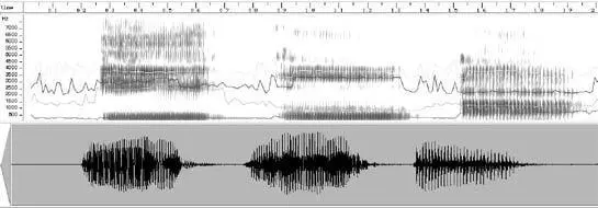
A spectrogram of three vowels. From left to right: [i] as in “appr e ciate,” [u] as in “aco u stic,” and [a] as in “ah.” The Y axis represents frequency of sound. The darker the band the more acoustic energy there is at that frequency.

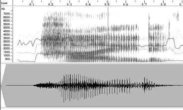
A spectrogram of a person saying the word “hide.” The horizontal lines show the formants, which are sustained frequencies that have especially high energy. 10

The result was partially successful. We could train our device to learn the patterns for a particular person using a moderate-sized vocabulary, measured in thousands of words. When we attempted to recognize tens of thousands of words, handle multiple speakers, and allow fully continuous speech (that is, speech with no pauses between words), we ran into the invariance problem. Different people enunciated the same phoneme differently—for example, one person’s “e” phoneme may sound like someone else’s “ah.” Even the same person was inconsistent in the way she spoke a particular phoneme. The pattern of a phoneme was often affected by other phonemes nearby. Many phonemes were left out completely. The pronunciation of words (that is, how phonemes are strung together to form words) was also highly variable and dependent on context. The linguistic rules we had programmed were breaking down and could not keep up with the extreme variability of spoken language.

It became clear to me at the time that the essence of human pattern and conceptual recognition was based on hierarchies. This is certainly apparent for human language, which constitutes an elaborate hierarchy of structures. But what is the element at the base of the structures? That was the first question I considered as I looked for ways to automatically recognize fully normal human speech.

Sound enters the ear as a vibration of the air and is converted by the approximately 3,000 inner hair cells in the cochlea into multiple frequency bands. Each hair cell is tuned to a particular frequency (note that we perceive frequencies as tones) and each acts as a frequency filter, emitting a signal whenever there is sound at or near its resonant frequency. As it leaves the human cochlea, sound is thereby represented by approximately 3,000 separate signals, each one signifying the time-varying intensity of a narrow band of frequencies (with substantial overlap among these bands).

Even though it was apparent that the brain was massively parallel, it seemed impossible to me that it was doing pattern matching on 3,000 separate auditory signals. I doubted that evolution could have been that inefficient. We now know that very substantial data reduction does indeed take place in the auditory nerve before sound signals ever reach the neocortex.

In our software-based speech recognizers, we also used filters implemented as software—sixteen to be exact (which we later increased to thirty-two, as we found there was not much benefit to going much higher than this). So in our system, each point in time was represented by sixteen numbers. We needed to reduce these sixteen streams of data into one while at the same emphasizing the features that are significant in recognizing speech.

We used a mathematically optimal technique to accomplish this, called vector quantization. Consider that at any particular point in time, sound (at least from one ear) was represented by our software by sixteen different numbers: that is, the output of the sixteen frequency filters. (In the human auditory system the figure would be 3,000, representing the output of the 3,000 cochlea inner hair cells.) In mathematical terminology, each such set of numbers (whether 3,000 in the biological case or 16 in our software implementation) is called a vector.

For simplicity, let’s consider the process of vector quantization with vectors of two numbers. Each vector can be considered a point in two-dimensional space.

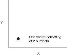
If we have a very large sample of such vectors and plot them, we are likely to notice clusters forming.

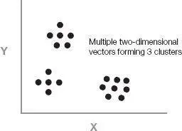
In order to identify the clusters, we need to decide how many we will allow. In our project we generally allowed 1,024 clusters so that we could number them and assign each cluster a 10-bit label (because 2 10= 1,024). Our sample of vectors represents the diversity that we expect. We tentatively assign the first 1,024 vectors to be one-point clusters. We then consider the 1,025th vector and find the point that it is closest to. If that distance is greater than the smallest distance between any pair of the 1,024 points, we consider it as the beginning of a new cluster. We then collapse the two (one-point) clusters that are closest together into a single cluster. We are thus still left with 1,024 clusters. After processing the 1,025th vector, one of those clusters now has more than one point. We keep processing points in this way, always maintaining 1,024 clusters. After we have processed all the points, we represent each multipoint cluster by the geometric center of the points in that cluster.

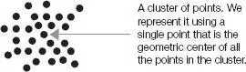
We continue this iterative process until we have run through all the sample points. Typically we would process millions of points into 1,024 (2 10) clusters; we’ve also used 2,048 (2 11) or 4,096 (2 12) clusters. Each cluster is represented by one vector that is at the geometric center of all the points in that cluster. Thus the total of the distances of all the points in the cluster to the center point of the cluster is as small as possible.

The result of this technique is that instead of having the millions of points that we started with (and an even larger number of possible points), we have now reduced the data to just 1,024 points that use the space of possibilities optimally. Parts of the space that are never used are not assigned any clusters.

We then assign a number to each cluster (in our case, 0 to 1,023). That number is the reduced, “quantized” representation of that cluster, which is why the technique is called vector quantization. Any new input vector that arrives in the future is then represented by the number of the cluster whose center point is closest to this new input vector.

We can now precompute a table with the distance of the center point of every cluster to every other center point. We thereby have instantly available the distance of this new input vector (which we represent by this quantized point—in other words, by the number of the cluster that this new point is closest to) to every other cluster. Since we are only representing points by their closest cluster, we now know the distance of this point to any other possible point that might come along.