Нассим Талеб - The Black Swan. The Impact of the Highly Improbable

Play one more round, the fourth. There will be sixteen equally likely outcomes. You will have one case of four wins, one case of four losses, four cases of two wins, four cases of two losses, and six break-even cases.

The quincunx (its name is derived from the Latin for five) in the pinball example shows the fifth round, with thirty-two possibilities, easy to track. Such was the concept behind the quincunx used by Francis Galton. Galton was both insufficiently lazy and a bit too innocent of mathematics; instead of building the contraption, he could have worked with simpler algebra, or perhaps undertaken a thought experiment like this one.

Let’s keep playing. Continue until you have forty flips. You can perform them in minutes, but we will need a calculator to work out the number of outcomes, which are taxing to our simple thought method. You will have about 1,099,511,627,776 possible combinations—more than one thousand billion. Don’t bother doing the calculation manually, it is two multiplied by itself forty times, since each branch doubles at every juncture. (Recall that we added a win and a lose at the end of the alternatives of the third round to go to the fourth round, thus doubling the number of alternatives.) Of these combinations, only one will be up forty, and only one will be down forty. The rest will hover around the middle, here zero.

We can already see that in this type of randomness extremes are exceedingly rare. One in 1,099,511,627,776 is up forty out of forty tosses. If you perform the exercise of forty flips once per hour, the odds of getting 40 ups in a row are so small that it would take quite a bit of forty-flip trials to see it. Assuming you take a few breaks to eat, argue with your friends and roommates, have a beer, and sleep, you can expect to wait close to four million lifetimes to get a 40-up outcome (or a 40-down outcome) just once. And consider the following. Assume you play one additional round, for a total of 41; to get 41 straight heads would take eight million lifetimes! Going from 40 to 41 halves the odds. This is a key attribute of the nonscalable framework to analyzing randomness: extreme deviations decrease at an increasing rate. You can expect to toss 50 heads in a row once in four billion lifetimes!

FIGURE 9: NUMBERS OF WINS TOSSED

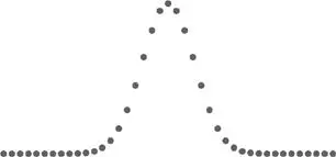
Result of forty tosses. We see the proto-bell curve emerging.

We are not yet fully in a Gaussian bell curve, but we are getting dangerously close. This is still proto-Gaussian, but you can see the gist. (Actually, you will never encounter a Gaussian in its purity since it is a Platonic form—you just get closer but cannot attain it.) However, as you can see in Figure 9, the familiar bell shape is starting to emerge.

How do we get even closer to the perfect Gaussian bell curve? By refining the flipping process. We can either flip 40 times for $1 a flip or 4,000 times for ten cents a flip, and add up the results. Your expected risk is about the same in both situations—and that is a trick. The equivalence in the two sets of flips has a little nonintuitive hitch. We multiplied the number of bets by 100, but divided the bet size by 10—don’t look for a reason now, just assume that they are “equivalent.” The overall risk is equivalent, but now we have opened up the possibility of winning or losing 400 times in a row. The odds are about one in 1 with 120 zeroes after it, that is, one in 1,000,000,000,000,000,000,000,000,000,000,000,000, 000,000,000,000,000,000,000,000,000,000,000,000,000,000,000,000, 000,000,000,000,000,000,000,000,000,000,000,000 times.

Continue the process for a while. We go from 40 tosses for $1 each to 4,000 tosses for 10 cents, to 400,000 tosses for 1 cent, getting close and closer to a Gaussian. Figure 10 shows results spread between −40 and 40, namely eighty plot points. The next one would bring that up to 8,000 points.

FIGURE 10: A MORE ABSTRACT VERSION: PLATO’S CURVE

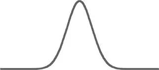
An infinite number of tosses.

Let’s keep going. We can flip 4,000 times staking a tenth of a penny. How about 400,000 times at 1/1000 of a penny? As a Platonic form, the pure Gaussian curve is principally what happens when he have an infinity of tosses per round, with each bet infinitesimally small. Do not bother trying to visualize the results, or even make sense out of them. We can no longer talk about an “infinitesimal” bet size (since we have an infinity of these, and we are in what mathematicians call a continuous framework). The good news is that there is a substitute.

We have moved from a simple bet to something completely abstract. We have moved from observations into the realm of mathematics. In mathematics things have a purity to them.

Now, something completely abstract is not supposed to exist, so please do not even make an attempt to understand Figure 10 . Just be aware of its use. Think of it as a thermometer: you are not supposed to understand what the temperature means in order to talk about it. You just need to know the correspondence between temperature and comfort (or some other empirical consideration). Sixty degrees corresponds to pleasant weather; ten below is not something to look forward to. You don’t necessarily care about the actual speed of the collisions among particles that more technically explains temperature. Degrees are, in a way, a means for your mind to translate some external phenomena into a number. Likewise, the Gaussian bell curve is set so that 68.2 percent of the observations fall between minus one and plus one standard deviations away from the average. I repeat: do not even try to understand whether standard deviation is average deviation —it is not, and a large (too large) number of people using the word standard deviation do not understand this point. Standard deviation is just a number that you scale things to, a matter of mere correspondence if phenomena were Gaussian .

These standard deviations are often nicknamed “sigma.” People also talk about “variance” (same thing: variance is the square of the sigma, i.e., of the standard deviation).

Note the symmetry in the curve. You get the same results whether the sigma is positive or negative. The odds of falling below −4 sigmas are the same as those of exceeding 4 sigmas, here 1 in 32,000 times.

As the reader can see, the main point of the Gaussian bell curve is, as I have been saying, that most observations hover around the mediocre, the mean, while the odds of a deviation decline faster and faster (exponentially) as you move away from the mean. If you need to retain one single piece of information, just remember this dramatic speed of decrease in the odds as you move away from the average. Outliers are increasingly unlikely. You can safely ignore them.

This property also generates the supreme law of Mediocristan: given the paucity of large deviations, their contribution to the total will be vanishingly small.

In the height example earlier in this chapter, I used units of deviations of ten centimeters, showing how the incidence declined as the height increased. These were one sigma deviations; the height table also provides an example of the operation of “scaling to a sigma” by using the sigma as a unit of measurement.