Pedro Domingos - The Master Algorithm - How the Quest for the Ultimate Learning Machine Will Remake Our World

Clearly, if Robby did know them, it would be smooth sailing: as in Naïve Bayes, each cluster would be defined by its probability (17 percent of the objects generated were toys), and by the probability distribution of each attribute among the cluster’s members (for example, 80 percent of the toys are brown). Robby could estimate these probabilities just by counting the number of toys in the data, the number of brown toys, and so on. But in order to do that, we would need to know which objects are toys. This seems like a tough nut to crack, but it turns out we already know how to do it as well. If Robby has a Naïve Bayes classifier and needs to figure out the class of a new object, all he needs to do is apply the classifier and compute the probability of each class given the object’s attributes. (Small, fluffy, brown, bear-like, with big eyes, and a bow tie? Probably a toy but possibly an animal.)

So Robby is faced with a chicken-and-egg problem: if he knew the objects’ classes, he could learn the classes’ models by counting, and if he knew the models, he could infer the objects’ classes. We seem to be stuck again, but far from it: just start by guessing a class for each object any way you want-even at random-and you’re off to the races. From those classes and the data, you can learn the class models; based on these models you can reinfer the classes and so on. At first sight this looks like a crazy scheme: it may never finish, circling forever between inferring the classes from the models and the models from the classes, and even if it does finish, there’s no reason to believe it will settle on meaningful clusters. But in 1977 a trio of Harvard statisticians (Arthur Dempster, Nan Laird, and Donald Rubin) showed that the crazy scheme actually works: every time we go around the loop, the cluster model gets better, and the loop ends when the model is a local maximum of the likelihood. They called this scheme the EM algorithm, where the E stands for expectation (inferring the expected probabilities) and the M for maximization (estimating the maximum-likelihood parameters). They also showed that many previous algorithms were special cases of EM. For example, to learn hidden Markov models, we alternate between inferring the hidden states and estimating the transition and observation probabilities based on them. Whenever we want to learn a statistical model but are missing some crucial information (e.g., the classes of the examples), we can use EM. This makes it one of the most popular algorithms in all of machine learning.

You might have noticed a certain resemblance between k -means and EM, in that they both alternate between assigning entities to clusters and updating the clusters’ descriptions. This is not an accident: k -means itself is a special case of EM, which you get when all the attributes have “narrow” normal distributions, that is, normal distributions with very small variance. When clusters overlap a lot, an entity could belong to, say, cluster A with a probability of 0.7 and cluster B with a probability of 0.3, and we can’t just decide that it belongs to cluster A without losing information. EM takes this into account by fractionally assigning the entity to the two clusters and updating their descriptions accordingly. If the distributions are very concentrated, however, the probability that an entity belongs to the nearest cluster is always approximately 1, and all we have to do is assign entities to clusters and average the entities in each cluster to obtain its mean, which is just the k -means algorithm.

So far we’ve only seen how to learn one level of clusters, but the world is, of course, much richer than that, with clusters within clusters all the way down to individual objects: living things cluster into plants and animals, animals into mammals, birds, fishes, and so on, all the way down to Fido the family dog. No problem: once we’ve learned one set of clusters, we can treat them as objects and cluster them in turn, and so on up to the cluster of all things. Alternatively, we can start with a coarse clustering and then further divide each cluster into subclusters: Robby’s toys divide into stuffed animals, constructions toys, and so on; stuffed animals into teddy bears, plush kittens, and so on. Children seem to start out in the middle and then work their way up and down. For example, they learn dog before they learn animal or beagle . This might be a good strategy for Robby, as well.

Discovering the shape of the data

Whether it’s data pouring into Robby’s brain through his senses or the click streams of millions of Amazon customers, grouping a large number of entities into a smaller number of clusters is only half the battle. The other half is shortening the description of each entity. The very first picture of Mom that Robby sees comprises perhaps a million pixels, each with its own color, but you hardly need a million variables to describe a face. Likewise, each thing you click on at Amazon provides an atom of information about you, but what Amazon would really like to know is your likes and dislikes, not your clicks. The former, which are fairly stable, are somehow immanent in the latter, which grow without limit as you use the site. Little by little, all those clicks should add up to a picture of your taste, in the same way that all those pixels add up to a picture of your face. The question is how to do the adding.

A face has only about fifty muscles, so fifty numbers should suffice to describe all possible expressions, with plenty of room to spare. The shape of the eyes, nose, mouth, and so on-the features that let you tell one person from another-shouldn’t take more than a few dozen numbers, either. After all, with only ten choices for each facial feature, a police artist can put together a sketch of a suspect that’s good enough to recognize him. You can add a few more numbers to specify lighting and pose, but that’s about it. So if you give me a hundred numbers or so, that should be enough to re-create a picture of a face. Conversely, Robby’s brain should be able to take in a picture of a face and quickly reduce it to the hundred numbers that really matter.

Machine learners call this process dimensionality reduction because it reduces a large number of visible dimensions (the pixels) to a few implicit ones (expression, facial features). Dimensionality reduction is essential for coping with big data-like the data coming in through your senses every second. A picture may be worth a thousand words, but it’s also a million times more costly to process and remember. Yet somehow your visual cortex does a pretty good job of whittling it down to a manageable amount of information, enough to navigate the world, recognize people and things, and remember what you saw. It’s one of the great miracles of cognition and so natural you’re not even conscious of doing it.

When you arrange books on a shelf so that books on similar topics are close to each other, you’re doing a kind of dimensionality reduction, from the vast space of topics to the one-dimensional shelf. Unavoidably, some books that are closely related will wind up far apart on the shelf, but you can still order them in a way that minimizes such occurrences. That’s what dimensionality reduction algorithms do.

Suppose I give you the GPS coordinates of all the shops in Palo Alto, California, and you plot a few of them on a piece of paper:

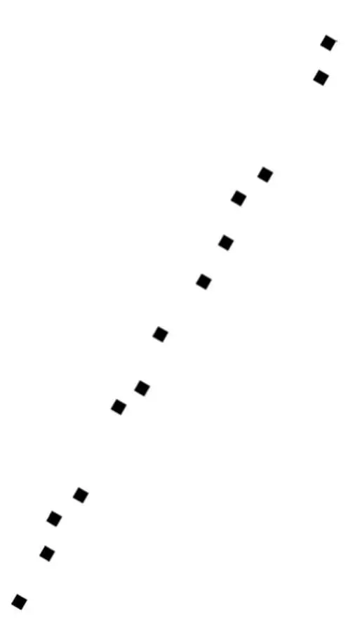
You can probably tell just by looking at this plot that the main street in Palo Alto runs southwest-northeast. You didn’t draw a street, but you can intuit that it’s there from the fact that all the points fall along a straight line (or close to it-they can be on different sides of the street). Indeed, the street is University Avenue, and if you want to shop or eat out in Palo Alto, that’s the place to go. As a bonus, once you know that the shops are on University Avenue, you don’t need two numbers to locate them, just one: the street number (or, if you wanted to be really precise, the distance from the shop to the Caltrain station, on the southwest corner, which is where University Avenue begins).