Pedro Domingos - The Master Algorithm - How the Quest for the Ultimate Learning Machine Will Remake Our World

To handle weakly relevant attributes, one option is to learn attribute weights. Instead of letting the similarity along all dimensions count equally, we “shrink” the less-relevant ones. Suppose the training examples are points in a room, and the height dimension is not that important for our purposes. Discarding it would project all examples onto the floor. Downweighting it is more like giving the room a lower ceiling. The height of a point still counts when computing its distance to other points, but less than its horizontal position. And like many other things in machine learning, we can learn attribute weights by gradient descent.

It may happen that the room has a high ceiling, but the data points are all near the floor, like a thin layer of dust settling on the carpet. In that case, we’re in luck: the problem looks three dimensional, but in effect it’s closer to two dimensional. We don’t have to shrink height because nature has already shrunk it for us. This “blessing of nonuniformity,” whereby data is not spread uniformly in (hyper) space, is often what saves the day. The examples may have a thousand attributes, but in reality they all “live” in a much lower-dimensional space. That’s why nearest-neighbor can be good for handwritten digit recognition, for example: each pixel is a dimension, so there are many, but only a tiny fraction of all possible images are digits, and they all live together in a cozy little corner of hyperspace. The shape of the lower-dimensional space the data lives in may be quite capricious, however. For example, if a room has furniture in it, the dust doesn’t just settle on the floor; it settles on the tabletops, chair seats, bed covers, and whatnot. If we can figure out the approximate shape of the blanket of dust covering the room, then all we need is each point’s coordinates on it. As we’ll see in the next chapter, there’s a whole subfield of machine learning dedicated to, so to speak, discovering blanket shapes by groping around in the darkness of hyperspace.

Snakes on a plane

Up until the mid-1990s, the most widely used analogical learner was nearest-neigbhor, but it was overshadowed by its more glamorous cousins from the other tribes. But then a new similarity-based algorithm burst onto the scene, sweeping all before it. In fact, you could say it was another “peace dividend” from the end of the Cold War. Support vector machines, or SVMs for short, were the brainchild of Vladimir Vapnik, a Soviet frequentist. Vapnik spent most of his career at the Institute of Control Sciences in Moscow, but in 1990, as the Soviet Union unraveled, he emigrated to the United States, where he joined the legendary Bell Labs. While in Russia, Vapnik had been mostly content to do theoretical, pencil-and-paper work, but the atmosphere at Bell Labs was different. Researchers were looking for practical results, and Vapnik finally decided to turn his ideas into an algorithm. Within a few years, he and his colleagues at Bell Labs had developed SVMs, and before long they were everywhere, setting new accuracy records left and right.

Superficially, an SVM looks a lot like weighted k -nearest-neighbor: the frontier between the positive and negative classes is defined by a set of examples and their weights, together with a similarity measure. A test example belongs to the positive class if, on average, it looks more like the positive examples than the negative ones. The average is weighted, and the SVM remembers only the key examples required to pin down the frontier. If you look back at the Posistan/Negaland example, once we throw away all the towns that aren’t on the border, all that’s left is this map:

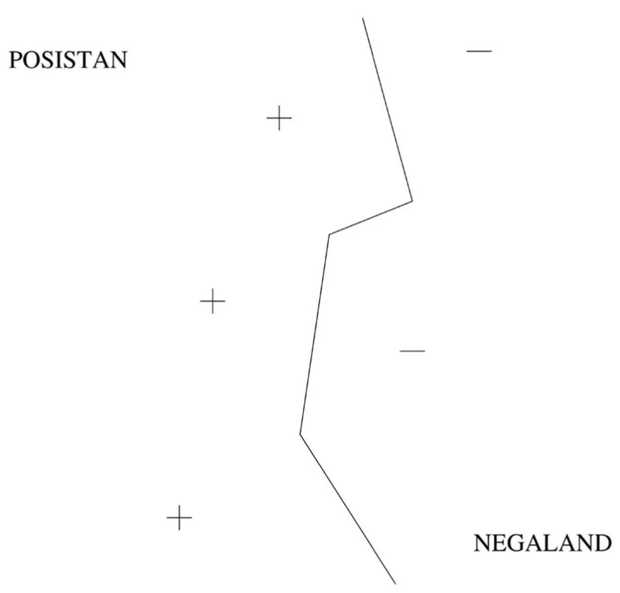
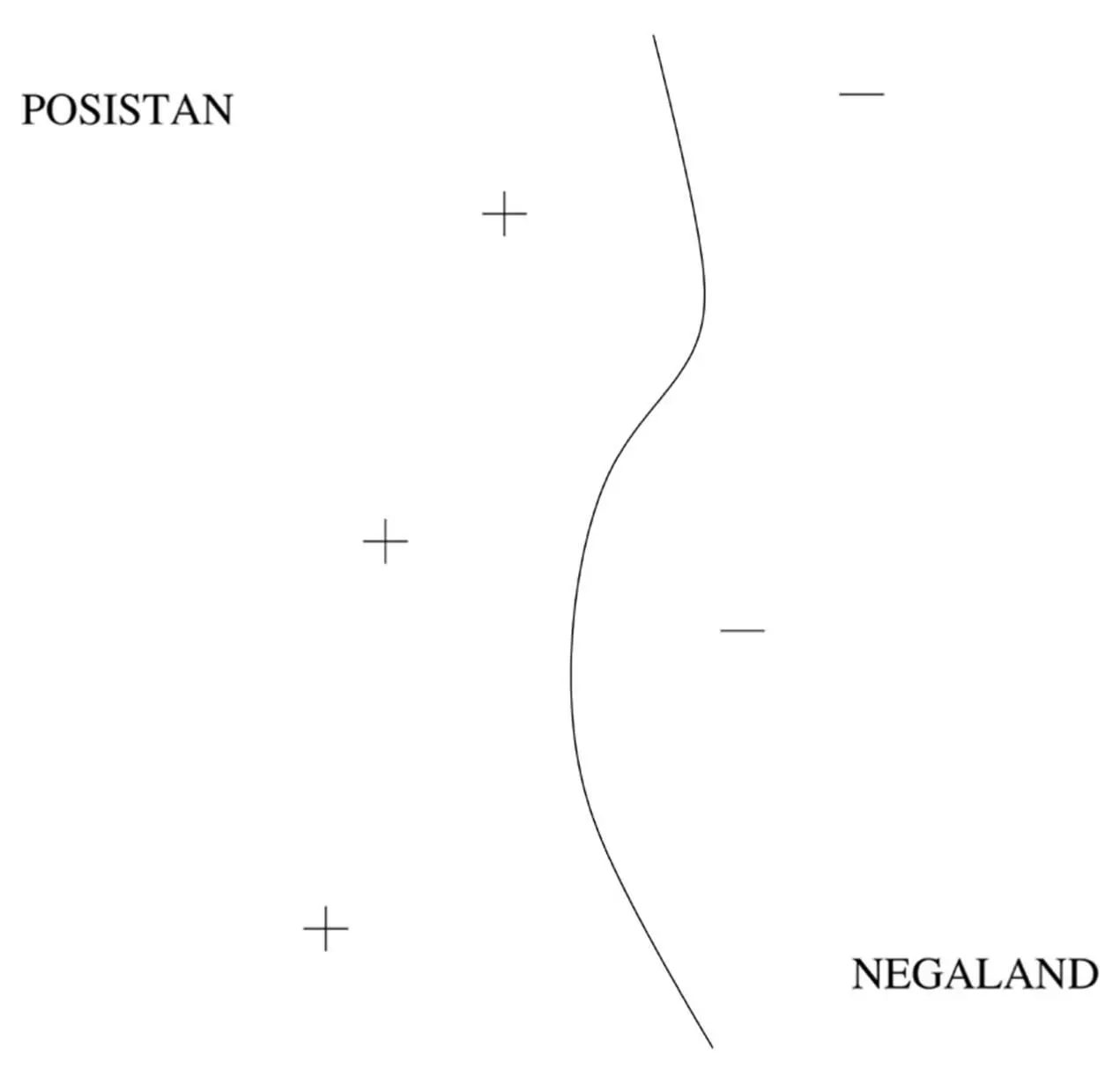
These examples are called support vectors because they’re the vectors that “hold up” the frontier: remove one, and a section of the frontier slides to a different place. You may also notice that the frontier is a jagged line, with sudden corners that depend on the exact location of the examples. Real concepts tend to have smoother borders, which means nearest-neighbor’s approximation is probably not ideal. But with SVMs, we can learn smooth frontiers, more like this:

To learn an SVM, we need to choose the support vectors and their weights. The similarity measure, which in SVM-land is called the kernel, is usually chosen a priori. One of Vapnik’s key insights was that not all borders that separate the positive training examples from the negative ones are created equal. Suppose Posistan and Negaland are at war, and they’re separated by a no-man’s-land with minefields on either side. Your mission is to survey the no-man’s-land, walking from one end of it to the other without stepping on any mines. Luckily, you have a map of where the mines are buried. Obviously, you don’t just take any old path: you give the mines the widest possible berth. That’s what SVMs do, with the examples as mines and the learned border as the chosen path. The closest the border ever comes to an example is its margin of safety, and the SVM chooses the support vectors and weights that yield the maximum possible margin. For example, the solid straight-line border in this figure is better than the dotted one:

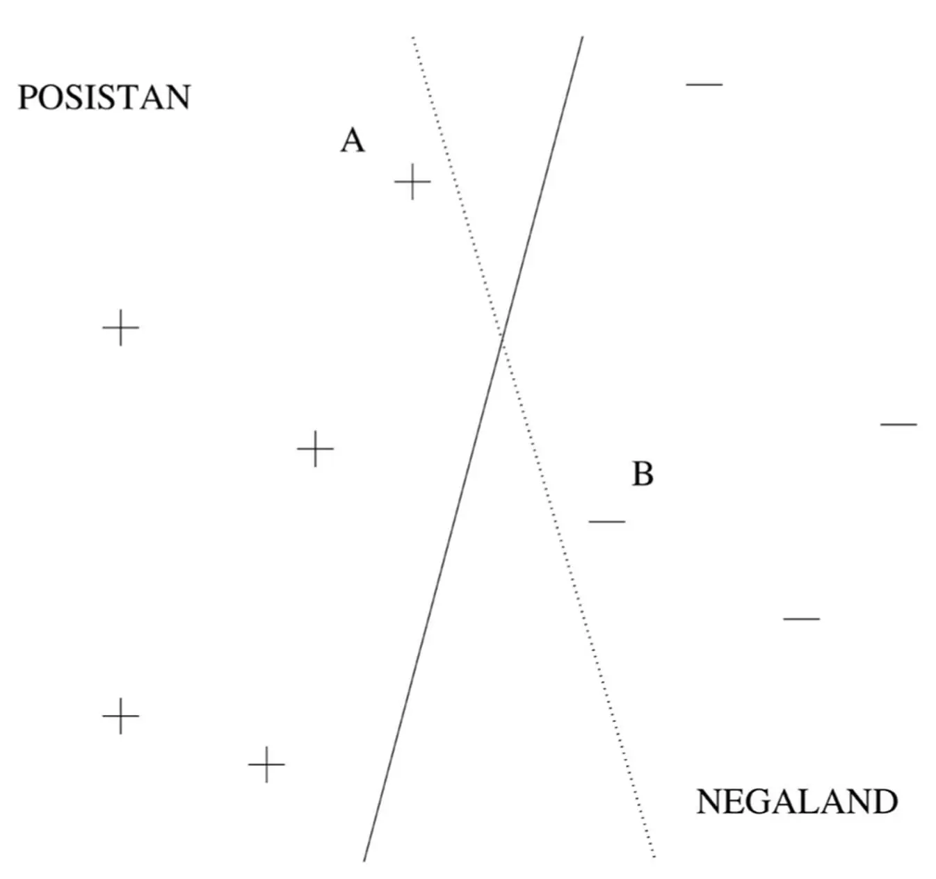
The dotted border separates the positive and negative examples just fine, but it comes dangerously close to stepping on the landmines at A and B. These examples are support vectors: delete one of them, and the maximum-margin border moves to a different place. In general, the border can be curved, of course, making the margin harder to visualize, but we can think of the border as a snake slithering down the no-man’s-land, and the margin is how fat the snake can be. If a very fat snake can slither all the way down without blowing itself to smithereens, then the SVM can separate the positive and negative examples very well, and Vapnik showed that in this case we can be confident that the SVM didn’t overfit. Intuitively, compared to a thin snake, there are fewer ways a fat snake can slither down while avoiding the landmines; and likewise, compared to a low-margin SVM, a high-margin one has fewer chances of overfitting by drawing an overly intricate border.

The second part of the story is how the SVM finds the fattest snake that fits between the positive and negative landmines. At first sight, it might seem like learning a weight for each training example by gradient descent would do the trick. All we have to do is find the weights that maximize the margin, and any examples that end up with zero weight can be discarded. Unfortunately, this would just make the weights grow without limit, because mathematically, the larger the weights, the larger the margin. If you’re one foot from a landmine and you double the size of everything including yourself, you are now two feet from the landmine, but that doesn’t make you any less likely to step on it. Instead, we have to maximize the margin under the constraint that the weights can only increase up to some fixed value. Or, equivalently, we can minimize the weights under the constraint that all examples have a given margin, which could be one-the precise value is arbitrary. This is what SVMs usually do.

Constrained optimization is the problem of maximizing or minimizing a function subject to constraints. The universe maximizes entropy subject to keeping energy constant. Problems of this type are widespread in business and technology. For example, we may want to maximize the number of widgets a factory produces, subject to the number of machine tools available, the widgets’ specs, and so on. With SVMs, constrained optimization became crucial for machine learning as well. Unconstrained optimization is getting to the top of the mountain, and that’s what gradient descent (or, in this case, ascent) does. Constrained optimization is going as high as you can while staying on the road. If the road goes up to the very top, the constrained and unconstrained problems have the same solution. More often, though, the road zigzags up the mountain and then back down without ever reaching the top. You know you’ve reached the highest point on the road when you can’t go any higher without driving off the road; in other words, when the path to the top is at right angles to the road. If the road and the path to the top form an oblique angle, you can always get higher by driving farther along the road, even if that doesn’t get you higher as quickly as aiming straight for the top of the mountain. So the way to solve a constrained optimization problem is to follow not the gradient but the part of it that’s parallel to the constraint surface-in this case the road-and stop when that part is zero.