Bhisham C. Gupta - Statistics and Probability with Applications for Engineers and Scientists Using MINITAB, R and JMP
Здесь есть возможность читать онлайн «Bhisham C. Gupta - Statistics and Probability with Applications for Engineers and Scientists Using MINITAB, R and JMP» — ознакомительный отрывок электронной книги совершенно бесплатно, а после прочтения отрывка купить полную версию. В некоторых случаях можно слушать аудио, скачать через торрент в формате fb2 и присутствует краткое содержание. Жанр: unrecognised, на английском языке. Описание произведения, (предисловие) а так же отзывы посетителей доступны на портале библиотеки ЛибКат.
- Название:Statistics and Probability with Applications for Engineers and Scientists Using MINITAB, R and JMP
- Автор:
- Жанр:
- Год:неизвестен
- ISBN:нет данных
- Рейтинг книги:4 / 5. Голосов: 1
-
Избранное:Добавить в избранное
- Отзывы:
-
Ваша оценка:
Statistics and Probability with Applications for Engineers and Scientists Using MINITAB, R and JMP: краткое содержание, описание и аннотация
Предлагаем к чтению аннотацию, описание, краткое содержание или предисловие (зависит от того, что написал сам автор книги «Statistics and Probability with Applications for Engineers and Scientists Using MINITAB, R and JMP»). Если вы не нашли необходимую информацию о книге — напишите в комментариях, мы постараемся отыскать её.
Statistics and Probability with Applications for Engineers and Scientists using MINITAB, R and JMP, Second Edition Features two new chapters—one on Data Mining and another on Cluster Analysis Now contains R exhibits including code, graphical display, and some results MINITAB and JMP have been updated to their latest versions Emphasizes the p-value approach and includes related practical interpretations Offers a more applied statistical focus, and features modified examples to better exhibit statistical concepts Supplemented with an Instructor's-only solutions manual on a book’s companion website
is an excellent text for graduate level data science students, and engineers and scientists. It is also an ideal introduction to applied statistics and probability for undergraduate students in engineering and the natural sciences.
Statistics and Probability with Applications for Engineers and Scientists Using MINITAB, R and JMP — читать онлайн ознакомительный отрывок
Ниже представлен текст книги, разбитый по страницам. Система сохранения места последней прочитанной страницы, позволяет с удобством читать онлайн бесплатно книгу «Statistics and Probability with Applications for Engineers and Scientists Using MINITAB, R and JMP», без необходимости каждый раз заново искать на чём Вы остановились. Поставьте закладку, и сможете в любой момент перейти на страницу, на которой закончили чтение.
Интервал:
Закладка:

Notes :
1 The IQR gives an estimate of the range of the middle 50% of the population.
2 The IQR is potentially a more meaningful measure of dispersion than the range as it is not affected by the extreme values that may be present in the data. By trimming 25% of the data from the bottom and 25% from the top, we eliminate the extreme values that may be present in the data set. Thus, the IQR is often used as a measure of comparison between two or more data sets on similar studies.
2.7.4 Coefficient of Variation
The coefficient of variation is usually denoted by  and is defined as the ratio of the standard deviation to the mean expressed as a percentage:
(2.7.4) 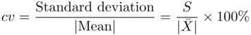
where  is the absolute value of the mean. The coefficient of variation is a relative comparison of a standard deviation to its mean and is unitless. The cv is commonly used to compare the variability in two populations. For example, we might want to compare the disparity of earnings for technicians who have the same employer but work in two different countries. In this case, we would compare the coefficient of variation of the two populations rather than compare the variances, which would be an invalid comparison. The population with a greater coefficient of variation, generally speaking, has more variability than the other. As an illustration, we consider the following example.
Example 2.7.3 A company uses two measuring instruments, one to measure the diameters of ball bearings and the other to measure the length of rods it manufactures. The quality control department of the company wants to find which instrument measures with more precision. To achieve this goal, a quality control engineer takes several measurements of a ball bearing by using one instrument and finds the sample average  and the standard deviation
  to be 3.84 and 0.02 mm, respectively. Then, he/she takes several measurements of a rod by using the other instrument and finds the sample average
  and the standard deviation
  to be 29.5 and 0.035 cm, respectively. Estimate the coefficient of variation from the two sets of measurements.
Solution:Using formula ( 2.7.4), we have


The measurements of the lengths of rod are relatively less variable than of the diameters of the ball bearings. Therefore, we can say the data show that instrument 2 is more precise than instrument 1.
Example 2.7.4 (Bus riders) The following data gives the number of persons who take a bus during the off‐peak time schedule (3–4 pm.) from Grand Central to Lower Manhattan in New York City. Using technology, find the numerical measures for these data:
| 17 | 12 | 12 | 14 | 15 | 16 | 16 | 16 | 16 | 17 | 17 | 18 | 18 | 18 | 19 | 19 | 20 | 20 | 20 | 20 |
| 20 | 20 | 20 | 20 | 21 | 21 | 21 | 22 | 22 | 23 | 23 | 23 | 24 | 24 | 25 | 26 | 26 | 28 | 28 | 28 |
MINITAB
1 Enter the data in column C1.
2 From the Menu bar, select Stat Basic Statistics Display Descriptive Statistics:
3 In the dialog box that appears, enter C1 under variables and select the option Statistics.
4 A new dialog box Descriptive Statistics: Statistics appears. In this dialog box, select the desired statistics and click OK in the two dialog boxes. The values of all the desired statistics as shown below will appear in the Session window.
USING R
We can use a few built in functions in R to get basic summary statistics. Functions ‘mean()’, ‘sd()’, and ‘var()’ are used to calculate the sample mean, standard deviation, and variance, respectively. The coefficient of variation can be calculated manually using the mean and variance results. The ‘quantile()’ function is used to obtain three quantiles and the minimum and maximum. The function ‘range()’ as shown below can be used to calculate the range of the data. The task can be completed by running the following R code in the R Console window.
x = c(17,12,12,14,15,16,16,16,16,17,17,18,18,18,19,19,20,20,20,20,20, 20,20,20,21,21,21,22,22,23,23,23, 24,24,25,26,26,28,28,28) #To concatenate resulting mean, standard deviation, variance, and coefficient of variation c(mean(x), sd(x), var(x), 100*sd(x)/mean(x))  20.125000 4.089934 16.727564 20.322656 #To obtain quartiles including min and max quantile(x)
| 0% | 25% | 50% | 75% | 100% |
| 12 | 17 | 20 | 23 | 28 |
#To obtain the range we find Max‐Min range(x)[2]‐range(x)[1]  16
16
2.8 Box‐Whisker Plot
In the above discussion, several times we made a mention of extreme values. At some point we may wish to know what values in a data set are extreme values, also known as outliers . An important tool called the box‐whisker plot or simply box plot , and invented by J. Tukey, helps us answer this question. Figure 2.8.1illustrates the construction of a box plot for any data set.
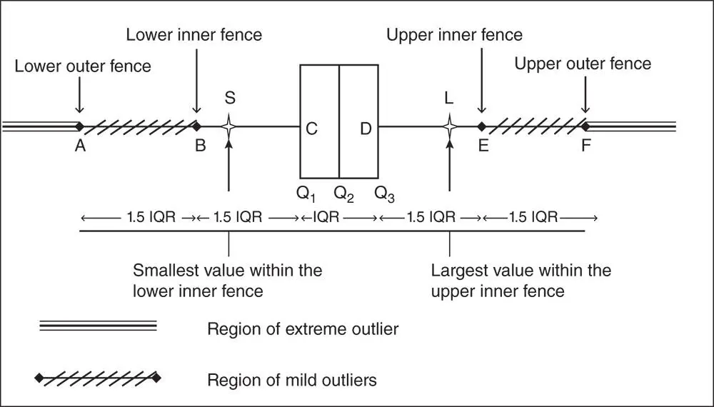
Figure 2.8.1Box‐whisker plot.
2.8.1 Construction of a Box Plot
1 Step 1. Find the quartiles , , and for the given data set.
2 Step 2. Draw a box with its outer lines of the box standing at the first quartile () and the third quartile (), and then draw a line at the second quartile (). The line at divides the box into two boxes, which may or may not be of equal size.
Читать дальшеИнтервал:
Закладка:
Похожие книги на «Statistics and Probability with Applications for Engineers and Scientists Using MINITAB, R and JMP»
Представляем Вашему вниманию похожие книги на «Statistics and Probability with Applications for Engineers and Scientists Using MINITAB, R and JMP» списком для выбора. Мы отобрали схожую по названию и смыслу литературу в надежде предоставить читателям больше вариантов отыскать новые, интересные, ещё непрочитанные произведения.


Обсуждение, отзывы о книге «Statistics and Probability with Applications for Engineers and Scientists Using MINITAB, R and JMP» и просто собственные мнения читателей. Оставьте ваши комментарии, напишите, что Вы думаете о произведении, его смысле или главных героях. Укажите что конкретно понравилось, а что нет, и почему Вы так считаете.