Chris Jones - End-to-end Data Analytics for Product Development
Здесь есть возможность читать онлайн «Chris Jones - End-to-end Data Analytics for Product Development» — ознакомительный отрывок электронной книги совершенно бесплатно, а после прочтения отрывка купить полную версию. В некоторых случаях можно слушать аудио, скачать через торрент в формате fb2 и присутствует краткое содержание. Жанр: unrecognised, на английском языке. Описание произведения, (предисловие) а так же отзывы посетителей доступны на портале библиотеки ЛибКат.
- Название:End-to-end Data Analytics for Product Development
- Автор:
- Жанр:
- Год:неизвестен
- ISBN:нет данных
- Рейтинг книги:3 / 5. Голосов: 1
-
Избранное:Добавить в избранное
- Отзывы:
-
Ваша оценка:
End-to-end Data Analytics for Product Development: краткое содержание, описание и аннотация
Предлагаем к чтению аннотацию, описание, краткое содержание или предисловие (зависит от того, что написал сам автор книги «End-to-end Data Analytics for Product Development»). Если вы не нашли необходимую информацию о книге — напишите в комментариях, мы постараемся отыскать её.
• Presents a guide to innovation feasibility and formulation and process development
• Contains the statistical tools used to solve challenges faced during product innovation and feasibility
• Offers information on stability studies which are common especially in chemical or pharmaceutical fields
• Includes a companion website which contains videos summarizing main concepts
Written for undergraduate students and practitioners in industry,
offers resources for the planning, conducting, analyzing and interpreting of controlled tests in order to develop effective products and processes.
End-to-end Data Analytics for Product Development — читать онлайн ознакомительный отрывок
Ниже представлен текст книги, разбитый по страницам. Система сохранения места последней прочитанной страницы, позволяет с удобством читать онлайн бесплатно книгу «End-to-end Data Analytics for Product Development», без необходимости каждый раз заново искать на чём Вы остановились. Поставьте закладку, и сможете в любой момент перейти на страницу, на которой закончили чтение.
Интервал:
Закладка:
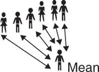
For numeric data, spread can also be measured by the variance . It accounts for all the data by measuring the distance or difference between each value and the mean . These differences are called deviations . The variance is the sum of squared deviations, divided by the number of values minus one. Roughly speaking, the variance (usually denoted by S 2) is the average of the squared deviations from the mean.
1 Example 1.2. Suppose you observed the following numeric data with their dotplot (Figure 1.9):
| 8.1 | 8.2 | 7.6 | 9.0 | 7.5 | 6.9 | 8.1 | 9.0 | 8.3 | 8.1 | 8.2 | 7.6 |

Figure 1.9 Dotplot.
The mean is equal to 8.05. Let's calculate the deviations from the mean and their squares:
| Deviations | Squared deviations |
| 8.1 − 8.05 = 0.05 | (0.05) 2= 0.0025 |
| 8.2 − 8.05 = 0.15 | (0.15) 2= 0.0225 |
| 7.6 − 8.05 = −0.45 | (−0.45) 2= 0.2025 |
| 9.0 − 8.05 = 0.95 | (0.95) 2= 0.9025 |
| 7.5 − 8.05 = −0.55 | (−0.55) 2= 0.3025 |
| 6.9 − 8.05 = −1.15 | (−1.15) 2= 1.3225 |
| 8.1 − 8.05 = 0.05 | (0.05) 2= 0.0025 |
| 9.0 − 8.05 = 0.95 | (0.95) 2= 0.9025 |
| 8.3 − 8.05 = 0.25 | (0.25) 2= 0.0625 |
| 8.1 − 8.05 = 0.05 | (0.05) 2= 0.0025 |
| 8.2 − 8.05 = 0.15 | (0.15) 2= 0.0225 |
| 7.6 − 8.05 = −0.45 | (−0.45) 2= 0.2025 |
Now, by adding up the squared deviations to get the sum and dividing it by the number of values minus one, you obtain the variance:
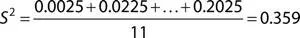
The variance measures how spread out the data are around their mean. The greater the variance, the greater the spread in the data.
The variance is not in the same units as the data, but in squared units. If the data are in grams, the variance is expressed in squared grams, and so on. Thus, for descriptive purposes, its square root, called standard deviation , is used instead.
The standard deviation (usually denoted by S) quantifies variability in the same units of measurement as we measure our data.
Considering the previous example, the standard deviation is:
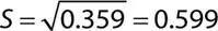
The greater the standard deviation, the greater the spread of data values around the mean.
Considering the mean and the standard deviation together and computing the range: mean ± S, we can say that data values vary on average from (mean − S) to (mean + S).
From the previous example the average range is:

The observed data vary on average from 7.5 to 8.6.
Stat Tool 1.10 Measures of Variability: Coefficient of Variation 
Another measure of variability for numeric data is the coefficient of variation .
It is calculated as follows:

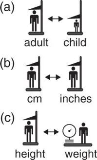
Being a dimensionless quantity, the coefficient of variation is a useful statistic for comparing the spread among several datasets, even if the means are different from one another (a), or data have different units (b), or data refer to different variables (c).
The higher the coefficient of variation, the higher the variability.
Stat Tool 1.11 Boxplots
So far, we have looked at three different aspects of numerical data analysis: shape of the data , central and non‐central tendency , and variability .
Boxplots can be used to assess and compare these three aspects of quantitative data distributions, and to look for outliers.
Like histograms, boxplots work best with moderate to large sample sizes (at least 20 values).
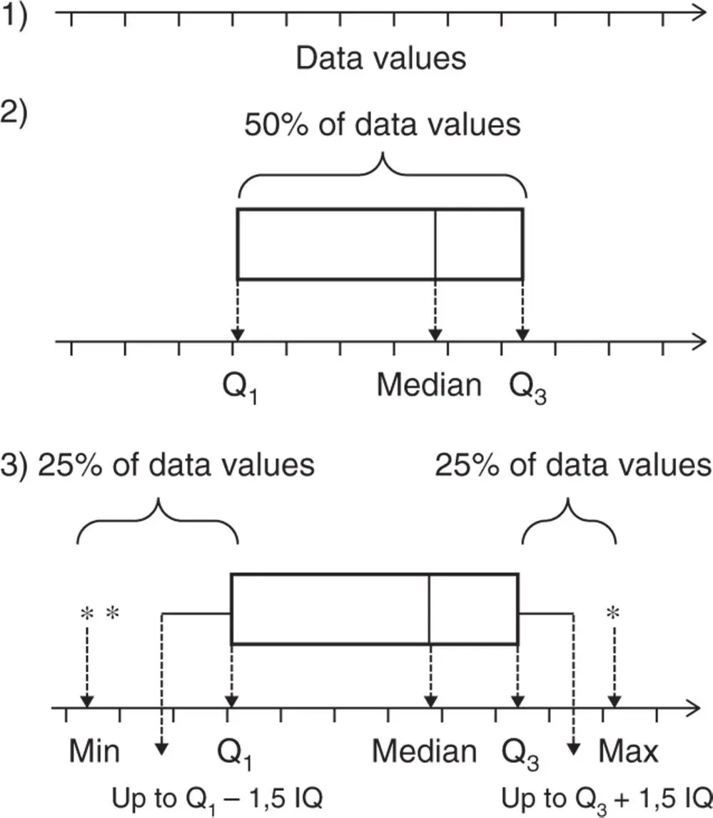
Let's look at how a boxplot is constructed. It can be displayed horizontally or vertically:
1 Start by drawing a horizontal or vertical axis in the units of the data values.
2 Draw a box to encompass 50% of middle data values. The left edge of the box is the first quartile Q1. The right edge of the box is the third quartile Q3. The width of the box is the interquartile range, IQR. Draw a line inside the box to denote the median.
3 Draw lines, called whiskers, on the left (to the minimum) and on the right (to the maximum) of the box to show the spread of the remaining data (25% of data points are below Q1 and 25% are above Q3). Several statistical softwares do not allow the whiskers to extend beyond one and a half times the interquartile range (1.5 × IQR). Any points outside of this range are outliers and are displayed individually by asterisks.
Boxplots help to summarize:
1 Central tendency. Look at the value of the median.
2 Non‐central tendency. Look at the values of the first quartile Q1 and the third quartile Q3.
3 Variability. Look at the length of the boxplot (range) and the width of the box (IQR).
4 Shape of data. Look at the position of the line of the median in the box and the position of the box between the two whiskers. In a symmetric distribution, the median is in the middle of the box and the two whiskers have the same length. In a skewed distribution, the median is closer to Q1 (skewed to the right) or to Q3 (skewed to the left) and the two whiskers do not have the same length (Figure 1.10).
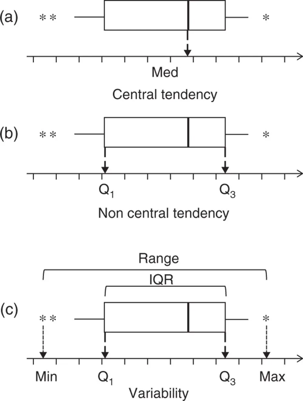
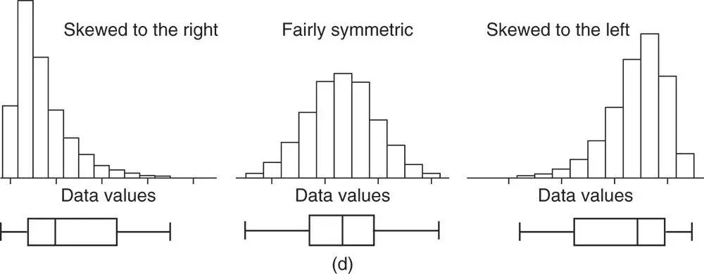
Figure 1.10 Histograms and boxplots.
Stat Tool 1.12 Basic Concepts of Statistical Inference
Интервал:
Закладка:
Похожие книги на «End-to-end Data Analytics for Product Development»
Представляем Вашему вниманию похожие книги на «End-to-end Data Analytics for Product Development» списком для выбора. Мы отобрали схожую по названию и смыслу литературу в надежде предоставить читателям больше вариантов отыскать новые, интересные, ещё непрочитанные произведения.


Обсуждение, отзывы о книге «End-to-end Data Analytics for Product Development» и просто собственные мнения читателей. Оставьте ваши комментарии, напишите, что Вы думаете о произведении, его смысле или главных героях. Укажите что конкретно понравилось, а что нет, и почему Вы так считаете.