Liuping Wang - PID Control System Design and Automatic Tuning using MATLAB/Simulink

1 In the IMC-PID controller tuning rules, if a faster closed-loop response is desired, would you increase or decrease the desired closed-loop time constant ?

2 For the tuning rules derived by Padula and Visioli, are there any closed-loop performance parameters chosen by the user?

3 Intuitively, would you increase the proportional controller gain if the PID controlled system is unstable when using the Padula and Visioli's tuning rules?

4 Would you increase the integral time constant if the PID controlled system is oscillatory when using the Padula and Visioli's tuning rules?

Several examples are presented in this section for evaluation of the tuning rules that are based on the first order plus delay model.

The first example is based on a first order plus delay plant and the second example is based a high order plant so that an approximation is made during the graphic procedure.

The unit step response of a continuous time transfer function model

(1.55)

is shown in Figure 1.15. Instead of using the first order plus delay model directly, we will find the PI controller parameters using the values of , , and delay .

Solution. A Simulink simulator is built to collect the step response testing data and to produce a figure for the step response. On this figure, a line is drawn to reflect the maximum slope of the reaction curve; there are two arrows marking the points of interest. Using MATLAB command ginput(2), with a click on the bottom point, we find the coordinates ; and with a click on the top point, we find .

From the readings of the two points, we find that

(1.56)

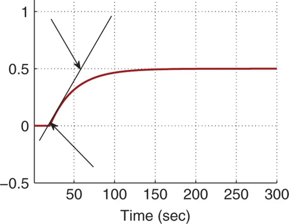
Figure 1.15Unit step response ( Example 1.6)

where is one since a unit step signal is used as the input. The time delay , and the parameter With these parameters, we calculate the PI controller parameters using the reaction curve based methods (see Tables 1.2, 1.3, and 1.6). The PI controller parameters are summarized in Table 1.7. Their closed-loop step responses are compared in Figure 1.16.

In reality, instead of a pure first order plus delay dynamics, there are more or less additional dynamics in the system. The tuning rules are applicable for a more complex system. We illustrate how to apply the tuning rules using the example below. This example also illustrates the fact that we need to be cautious when applying the tuning rules and be aware of their limitations.

Table 1.7PI controller parameters with reaction curve.

Ziegler–Nichols		3.1714		63
Cohen–Coon		3.3381		32.7131
Wang–Cluett		2.0571		41.4811

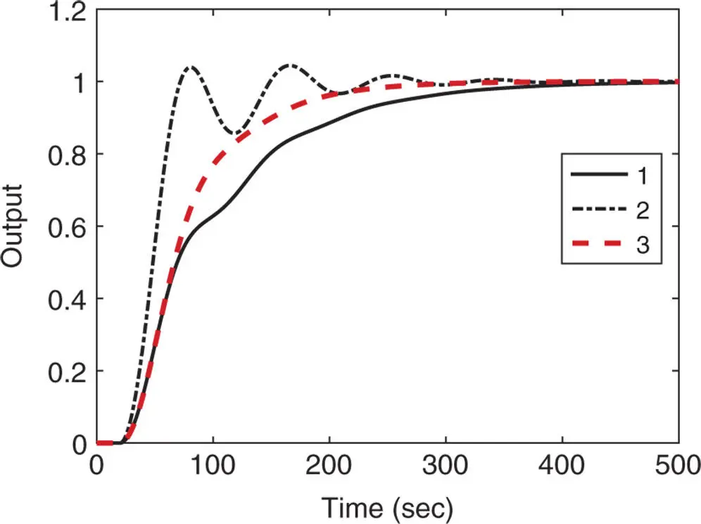
Figure 1.16Closed-loop unit step response with PI controller ( Example 1.6). Key: line (1) Ziegler–Nichols tuning rule; line (2) Cohen–Coon tuning rule; line (3) Wang–Cluett tuning rule.

A continuous time plant has the transfer function:

(1.57)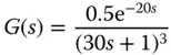

The unit step response of this transfer function model is shown in Figure 1.17. In this figure, a line is drawn to reflect the maximum slope of the reaction curve and the points of interest are marked by two arrows.

Using MATLAB command ginput(2), with a click on the bottom point, we will find the coordinates ; and a click on the top point, we will find . Find the PI and PID controllers using the reaction curve based tuning rules.

Solution. The steady state gain The time delay is and the parameter The PI controller parameters are calculated using the reaction curve based methods (see Tables 1.2, 1.3, and 1.6) and are summarized in Table 1.8. The closed-loop control systems with the PI controllers are simulated using the plant model (1.57). The unit closed-loop step responses are shown in Figure 1.18. From this figure, we can see that both PI controllers from Ziegler–Nichols and Cohen–Coon tuning rules failed to produce a stable closed-loop system. However, the PI controller using Wang–Cluett tuning rule gives a stable closed-loop system.

The PI control systems will be subsequently used as examples for closed-loop stability analysis. The Nyquist plots of the PI controllers used in this example are analyzed in Example 2.3 of Chapter 2.

The following example illustrates the applications of the Padula and Visioli tuning rules.

Figure 1.17Unit step response ( Example 1.7).

Table 1.8PI controller parameters with reaction curve.

Ziegler–Nichols		6.4		108
Cohen–Coon		6.5667		75.9231
Wang–Cluett		3.8867		127.2154

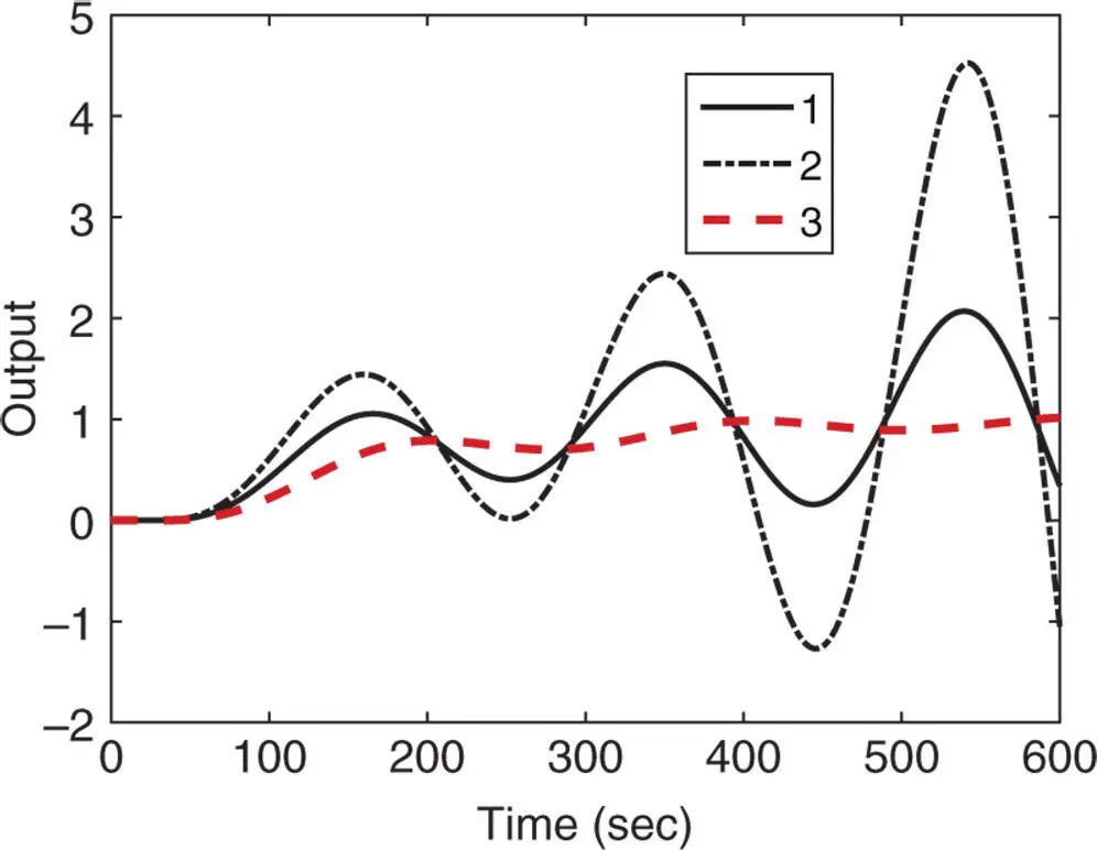
Figure 1.18Closed-loop unit step response with PI controller ( Example 1.7). Key: line (1) Ziegler–Nichols tuning rule; line (2) Cohen–Coon tuning rule; line (3) Wang–Cluett tuning rule.

Consider the same third order system with time delay used in Example 1.7. Find the PI and PID controller parameters using Padula and Visioli tuning rules and simulate their closed-loop step response.

Solution. The parameters used in the tuning rules are , , and . To evaluate the PI controller performance, Table 1.4 is used to calculate the controller parameters. For , we have and . For , we have and .