Doruk Senkal - Whole-Angle MEMS Gyroscopes

In the whole‐angle mechanization, the two modes of the gyroscope are allowed to freely oscillate and external forcing is only applied to null the effects of imperfections such as damping and asymmetry. In this mode of operation the mechanical element acts as a “mechanical integrator” of angular velocity, resulting in an angle measuring gyroscope, also known as a Rate Integrating Gyroscope (RIG).

Whole‐angle gyroscope architectures can be divided into three main categories based on the geometry of the resonator element: (i) lumped mass systems, (ii) ring/disk systems, and (iii) micro‐wineglasses. Ring/disk systems are further divided into three categories: (i) rings, (ii) concentric ring systems, and (iii) disks. Whereas, micro‐wineglasses are divided into two categories according to fabrication technology: surface micro‐machined and bulk micro‐machined wineglass gyroscope architectures, Figure 1.2[2].

String and bar resonators can also be instrumented to be used as whole‐angle gyroscopes, even though these types of mechanical elements are typically not used at micro‐scale due to limited transduction capacity. In principle, any axisymmetric elastic member can be instrumented to function as a whole‐angle gyroscope.

Gyroscopes are susceptible to a variety of error sources caused by a combination of inherent physical processes as well as external disturbances induced by the environment.

Error sources in a single axis rate gyroscope can be generalized according to the following formula:

(1.1)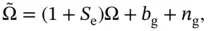

where is the measured gyroscope output, is scale factor error, is bias error, and is noise. Without loss of generality, for a whole‐angle gyroscope the error sources can be written as:

(1.2)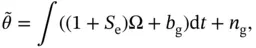

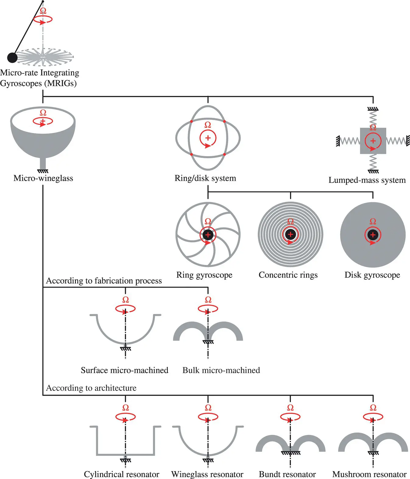
Figure 1.2 Micro‐rate integrating gyroscope (MRIG) architectures.

where is the measured gyroscope output, corresponding to total angular read‐out, including the actual angle of rotation, errors in scale factor, bias, and noise.

Scale factor (or sensitivity) errors represent a deviation in gyroscope sensitivity from expected values, which results in a nonunity gain between “true” angular rate and “perceived” angular rate. Scale factor errors can be caused by either an error in initial scale factor calibration or a drift in scale factor postcalibration due to a change in environmental conditions, such as a change in temperature or supply voltages, application of external mechanical stresses to the sensing element, or aging effects internal to the sensor, such as a change in cavity pressure of the vacuum packaged sensing element.

Bias (or offset) errors can be summarized as the deviation of time averaged gyroscope output from zero when there is no angular rate input to the sensor. Aside from initial calibration errors, bias errors can be caused by a change in environment conditions. Examples include a change in temperature, supply voltages or cavity pressure, aging of materials, and application of external mechanical stresses to the sensing element. An additional source of bias errors is external body loads, such as quasi‐static acceleration, as well as vibration.

Noise in gyroscopes can be grouped under white noise, flicker ( ) noise, and quantization noise. The most common numerical tool for representing gyroscope noise processes is Allan Variance.

Originally created to analyze frequency stability of clocks and oscillators, Allan Variance analysis is also widely used to represent various noise processes present in inertial sensors, such as gyroscopes [3]. Allan Variance analysis consists of data acquisition of gyroscope output over a period of time at zero rate input and constant temperature. This is followed by binning the data into groups of different integration times:

(1.3)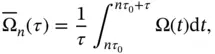

where is the sampling time, is the sample number, and is the bin size. The uncertainty between bins of same integration times is calculated using ensemble average:

(1.4)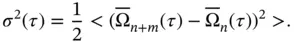

Finally, the calculated uncertainty with respect to integration time ( ) is plotted to reveal information about various noise processes within the gyroscope, Figure 1.3. Sections of the Allan Variance curve and their physical meaning is summarized below [3]:

Quantization noise is due to the conversion of gyroscope output from analog (continuous) signal to digital (countable) signal by Analog‐to‐Digital Converters (quantization). Quantization noise has a slope of on the Allan variance graph.

Angle Random Walk (ARW) is caused by white thermomechanical and thermoelectrical noise within the gyroscope, shows up with a slope of . It is usually reported using units (degrees per square root of hour) or (millidegrees per second per square root of hertz).

Rate Random Walk (RRW) is the random drift term within the gyroscope, shows up with a slope of opposite of ARW.

Bias instability is the lowest point of the Allan variance curve, shows up with a slope of zero. It represents the minimum detectable rate input within the gyroscope and is reported using units (degrees per hour) or (millidegrees per second). Bias instability is limited by a combination of flicker () noise, ARW, and RRW. Figure 1.3 Sample Allan variance analysis of gyroscope output, showing error in gyroscope output (deg/h or deg/s)with respect to integration time (s).