A. Gouveia Oliveira - Biostatistics Decoded

Figure 1.16 Properties of means and variances. Figure 1.17 Table of mean and variance properties. Figure 1.18 Tabulation of nominal data. Figure 1.19 Typical presentation of several nominal attributes in a single t... Figure 1.20 Tabulation of ordinal and interval data. Figure 1.21 Table with summary statistics describing the information collect... Figure 1.22 Illustration of the phenomenon of sampling variation. Above are ... Figure 1.23 Frequency distributions of some biological variables. Figure 1.24 The origin of the normal distribution. Figure 1.25 Frequency distribution of sums of identical variables with unifo... Figure 1.26 Properties of the normal distribution. Figure 1.27 Relationship between the area under the normal curve and the sta... Figure 1.28 The total obtained from the throw of six dice may be seen as the... Figure 1.29 Distribution of sample means of different sample sizes. Figure 1.30 Comparison of the computation of sample and population statistic... Figure 1.31 Illustration of the phenomenon of sampling variation. Above, pie... Figure 1.32 Probability distribution of a proportion: the binomial distribut... Figure 1.33 The convergence of the binomial to the normal distribution.

2 Chapter 2 Figure 2.1 The path to causality. Types of research studies. Figure 2.2 Classification of descriptive studies and corresponding populatio... Figure 2.3 Schema of a prevalence study. Figure 2.4 Steps in the inference of the value of the population mean from t... Figure 2.5 Statistical table of the normal distribution I. Figure 2.6 Statistical table of the normal distribution II. Figure 2.7 Relationship between the sample size and the spread of the sample... Figure 2.8 The error in the determination of confidence limits from standard... Figure 2.9 Several Student’s t distributions with different degrees of freed... Figure 2.10 Number of estimated standard errors on each side of the mean tha... Figure 2.11 Steps in the construction of 95% confidence intervals using Stud... Figure 2.12 Example of utilization of a statistical table of Student’s t dis... Figure 2.13 Steps in the construction of the 95% confidence interval of the ... Figure 2.14 Example of a statistical table of the binomial distribution. Figure 2.15 Relationship between sample size requirements and desired error ... Figure 2.16 Types of events. Figure 2.17 Organization of an incidence study. Figure 2.18 Schema of a cohort study. Figure 2.19 Closed and open cohort. Horizontal lines represent subjects obse... Figure 2.20 Illustration of the person‐time method. Figure 2.21 Illustration of the person‐time method applied to an event that ... Figure 2.22 The direct standardization method. Figure 2.23 The indirect standardization method. Figure 2.24 Time‐to‐event data. Figure 2.25 The actuarial method. Figure 2.26 Illustration of the actuarial method showing on the left the stu... Figure 2.27 Actuarial curve. Figure 2.28 Illustration of the Kaplan–Meier method showing on the left the ... Figure 2.29 Kaplan–Meier curve. Figure 2.30 Kaplan–Meier curve with 95% confidence bands. Figure 2.31 Representation of simple and systematic sampling. Each square re... Figure 2.32 Comparison of the binomial and the hypergeometric distributions.... Figure 2.33 Decreasing variance by splitting the population into strata. Figure 2.34 The different types of stratified sampling. Figure 2.35 Sample size requirements for simple and stratified sampling.Figure 2.36 Multistage and cluster sampling.Figure 2.37 Illustration of two‐stage sampling combined with sampling with p...

3 Chapter 3Figure 3.1 Data from a prevalence study of COPD in the general population.Figure 3.2 Probability distributions of proportions, odds, and logits.Figure 3.3 Attributable fraction in the population and among the exposed.Figure 3.4 Classification of observational analytical studies.Figure 3.5 Schema of an uncontrolled cross‐sectional analytical study. Black...Figure 3.6 Schema of an uncontrolled analytical cohort study. Black subjects...Figure 3.7 Models of the relationship between exposure and outcome. In (a), ...Figure 3.8 Schema of a case–control study. Black subjects are the exposed.Figure 3.9 Schema of a cohort study. Black subjects are the cases.Figure 3.10 Steps in the construction of 95% confidence intervals for the di...Figure 3.11 Steps in the construction of 95% confidence intervals for the di...Figure 3.12 Steps in the construction of 95% confidence intervals for the di...

4 Chapter 4Figure 4.1 Rationale of the z ‐test for large samples.Figure 4.2 Finding the exact p ‐value using a statistical table of the normal...Figure 4.3 The rationale of Student’s t ‐test in the case of small samples.Figure 4.4 Using the table of the t distribution to find exact p ‐values.Figure 4.5 Observed and expected frequencies under H 0.Figure 4.6 The chi‐square distribution under the null hypothesis for a 2 × 2...Figure 4.7 The chi‐square distribution with 1 to 10 degrees of freedom. The ...Figure 4.8 Statistical table of the chi‐square distribution.Figure 4.9 Observations in three samples of distinct populations (left panel...Figure 4.10 Procedure of ANOVA.Figure 4.11 Procedure of ANOVA with unequal sample sizes.Figure 4.12 Left ventricular ejection fraction in three groups classified ac...Figure 4.13 The F distribution with 2 and 90 degrees of freedom. The dark ar...Figure 4.14 Section of a statistical table of the F distribution.Figure 4.15 ANOVA table of the data of Figure 4.12.

5 Chapter 5Figure 5.1 Difference between two‐sided and one‐sided tests.Figure 5.2 Distribution of differences between sample means under a one‐side...Figure 5.3 The alpha and beta errors of a statistical test.Figure 5.4 Distribution of the differences between sample means under the nu...Figure 5.5 Effect of increasing sample size ratios on the statistical power ...Figure 5.6 Comparison of the distribution of the differences between means u...Figure 5.7 Commonly used transformations to the normal distribution.Figure 5.8 Rationale of a non‐parametric test for comparing two independent ...

6 Chapter 6Figure 6.1 Representation of the relationship between two interval variables...Figure 6.2 Rationale of the least squares method I.Figure 6.3 Rationale of the least squares method II.Figure 6.4 Rationale of the least‐squares method III.Figure 6.5 Sampling variation of the intercepts and slopes of regression lin...Figure 6.6 The slope m of a line connecting to an observation ( x , y ) is 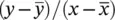....Figure 6.7 Steps in the calculation of the standard error of the regression ...Figure 6.8 Scatterplots with regression lines illustrating different situati...Figure 6.9 Illustration of the relationship between the total variance of Y ...Figure 6.10 Under H 0the variance of Y accounts for the difference ( y − y *...Figure 6.11 Regression analysis of FVC on height.Figure 6.12 Multiple regression analysis of FVC on sex adjusted for height t...Figure 6.13 Multiple regression analysis of FVC on two predictors.Figure 6.14 Residual plot of the regression of FVC on height and age.Figure 6.15 Patterns in residual plots suggestive of non‐normality of the re...Figure 6.16 Influence of an outlier (open circle) on the regression estimate...Figure 6.17 Results of the regression of FVC on three dummy variables encodi...Figure 6.18 Results of the regression of PEF on sex and height.Figure 6.19 Scatterplot of the data of the regression of PEF on sex and heig...Figure 6.20 Results of the regression of PEF on sex and height with a term f...Figure 6.21 Exemplification of an interaction effect on the relationship of ...Figure 6.22 Comparison of models obtained by linear regression (top) and pol...

Читать дальше