Yong Bai - Deepwater Flexible Risers and Pipelines
Здесь есть возможность читать онлайн «Yong Bai - Deepwater Flexible Risers and Pipelines» — ознакомительный отрывок электронной книги совершенно бесплатно, а после прочтения отрывка купить полную версию. В некоторых случаях можно слушать аудио, скачать через торрент в формате fb2 и присутствует краткое содержание. Жанр: unrecognised, на английском языке. Описание произведения, (предисловие) а так же отзывы посетителей доступны на портале библиотеки ЛибКат.

- Название:Deepwater Flexible Risers and Pipelines
- Автор:
- Жанр:
- Год:неизвестен
- ISBN:нет данных
- Рейтинг книги:4 / 5. Голосов: 1
-
Избранное:Добавить в избранное
- Отзывы:
-
Ваша оценка:
Deepwater Flexible Risers and Pipelines: краткое содержание, описание и аннотация
Предлагаем к чтению аннотацию, описание, краткое содержание или предисловие (зависит от того, что написал сам автор книги «Deepwater Flexible Risers and Pipelines»). Если вы не нашли необходимую информацию о книге — напишите в комментариях, мы постараемся отыскать её.
,, has been created to meet the needs of engineers and scientists to keep them up to date and informed of all of these advances. This second volume in the series focuses on flexible pipelines, risers, and umbilicals, offering the engineer the most thorough coverage of the state-of-the-art available. The authors of this work have written numerous books and papers on these subjects and are some of the most influential authors on flexible pipes in the world, contributing much of the literature on this subject to the industry. This new volume is a presentation of some of the most cutting-edge technological advances in technical publishing.
The first volume in this series, published by Wiley-Scrivener, is
, available at www.wiley.com. Laying the foundation for the series, it is a groundbreaking work, written by some of the world’s foremost authorities on pipes and pipelines. Continuing in this series, the editors have compiled the second volume, equally as groundbreaking, expanding the scope to pipelines, risers, and umbilicals.
This is the most comprehensive and in-depth series on pipelines, covering not just the various materials and their aspects that make them different, but every process that goes into their installation, operation, and design. This is the future of pipelines, and it is an important breakthrough. A must-have for the veteran engineer and student alike, this volume is an important new advancement in the energy industry, a strong link in the chain of the world’s energy production
Deepwater Flexible Risers and Pipelines — читать онлайн ознакомительный отрывок
Ниже представлен текст книги, разбитый по страницам. Система сохранения места последней прочитанной страницы, позволяет с удобством читать онлайн бесплатно книгу «Deepwater Flexible Risers and Pipelines», без необходимости каждый раз заново искать на чём Вы остановились. Поставьте закладку, и сможете в любой момент перейти на страницу, на которой закончили чтение.
Интервал:
Закладка:
When the imperfection is considered, the initial value of ovalization taken into account is1 = 0. 002, as minimum requirement, so that the initial displacement can be computed using Eq. (2.3), and it is equal to uR1 = 0.1652, referring the computation to the external radius. The outcomes of the theoretical model can be finally plotted, as shown in Figure 2.14, against the dimensionless load and for the ovality computed for each load increment as follows:
(2.16) 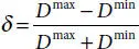
where, D maxand D minare the maximum and minimum diameters uploaded step by step from the results of the of the displacements, along x and y directions, respectively.
In the same way, outcomes for finite element model are computed extracting U1 and U2 and they are plotted in Figure 2.12. As previously said, it can be seen that the external surface displays different magnitude of displacements along x and y directions, as shown in Figures 2.10and 2.11.
As it was shown by Gay [7], the pre-buckling behaviors match one to each other with very low error. In Figure 2.14, it can be observed that for small value of external pressure the ovality increases linearly. In this phase, the very small difference between theoretical and numerical models can be caused by the fact that the theoretical model regards as an equivalent ring. Vice versa, the actual geometry shows gaps among the different parts, so it is obvious that results show a slightly different about stiffness. When the pressure increases, a non-linear trend is illustrated for both models. Numerical results show wider ovality for the same load, compared to analytical outcomes because of theoretical limits that consider as critical load the one for the case with no imperfections. As it was expected, the comparison between results makes sense in order to understand the pre-buckling behavior in terms of displacements and not in terms of collapse load. In fact, from Figure 2.12, the relevant output that comes out, in terms of pressure, is an error equal to 36% between theoretical and numerical outcomes when dealing with imperfections Table 2.3.
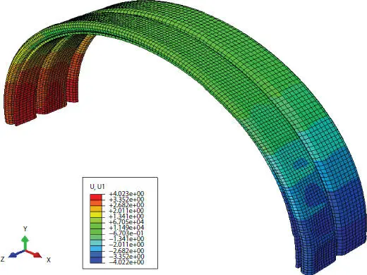
Figure 2.10 U1 displacements.
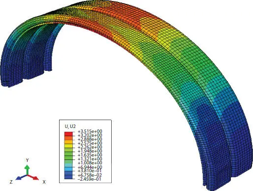
Figure 2.11 U2 displacements.
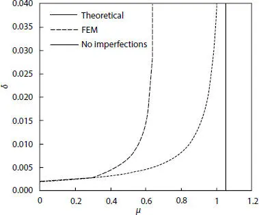
Figure 2.12 Ovality versus dimensionless load.
Table 2.3 Collapse pressures.
| Model | Collapse pressure [MPa] |
|---|---|
| No imperfections | 13.89 |
| Theoretical | 13.19 |
| FEM | 8.43 |
Moreover, here, it can be confirmed that, for a value of ovality equal to 4%, the external pressure no longer increases, while the ovality keep to sharply rise, so that it can be confirmed that L can be regarded as point of instability.
Eq. (2.6)in its original form, considers critical load for a ring without imperfection ( pcr ), in fact, the collapse is reached asymptotically for the latter value. In order to give reason to the similitude in terms of buckling pressure, the comparison of a series of both numerical and theoretical simulations is needed, keeping the bending stiffness of the cross-section constant and varying the radius of the pipe. The resolution of new pcr exhibits a valid formulation which guarantees theoretical results closer to the actuals and so to the FEM outcomes, which works in terms of both displacements and collapse pressure.
The available theoretical formulation which is based on thin-wall hypothesis gives results with lower error for high values of D/t. On the contrary, the gap between theoretical and numerical outcomes rises as the ratio under analysis decreases, which is captured in Figure 2.13. Thus, from this behavior, the consequence of considering zero error for high D/t ratios and justify the following assumption for the theoretical model.
An overall of eight models are analyzed for the same carcass cross-section and material, while different D/t ratios. In Figure 2.14, the collapse loads are plotted against different geometries when they reach the ovality limit. As it was expected, the critical buckling loads decreases as the tube diameters increase. Moreover, it is possible to see the asymptotic behavior between numerical and theoretical results for growing D/t ratios.
With that being said, the hypothesis of considering zero error for D/t = 30, which is the widest geometry considered. The choice to stop the computation at that value is made because it is rare to contemplate higher diameter configurations for deep water environments. Moreover, even if the error goes to zero asymptotically, as shown in Figure 2.15, this assumption wants to be a conservative suggestion since considering it for higher D/t standards will lead to a higher collapse pressure for the case under analysis.
Once the error is eliminated, the actual collapse loads accounting for imperfections can be obtained, and their behavior is shown in Figure 2.16.
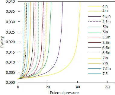
Figure 2.13 Ovality versus load for different geometries, where dashed lines stand for numerical results and continuous line stand for theoretical results.
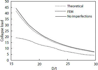
Figure 2.14 Critical loads versus dimensionless diameters.
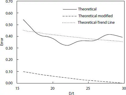
Figure 2.15 Error trend.
The extracted polynomial trend line depicts the guideline for the new theoretical model, and has the following formulation:
(2.17) 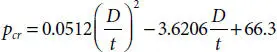
Eq. (2.17)is an estimation of the collapse pressure valid for the initial imperfection considered. It shows conservative results and it obviates the employment of the buckling load for the perfect ring, in the theoretical model, which leads to underestimation of collapse conditions.
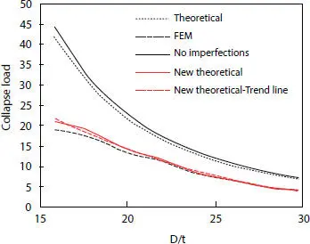
Figure 2.16 Critical load comparison for all the model established versus dimensionless diameters.
In order to get a behavior closer to the actual, Eq. (2.7)is developed again exploiting Eq. (2.16)as theoretical derivation to get the critical buckling load, which, for the case with D = 6 in, produces pcr = 9.12 MPa. As previously done, dimensionless load and ovality are plotted for both theoretical and numerical models, as shown in Figure 2.17.
Читать дальшеИнтервал:
Закладка:
Похожие книги на «Deepwater Flexible Risers and Pipelines»
Представляем Вашему вниманию похожие книги на «Deepwater Flexible Risers and Pipelines» списком для выбора. Мы отобрали схожую по названию и смыслу литературу в надежде предоставить читателям больше вариантов отыскать новые, интересные, ещё непрочитанные произведения.


Обсуждение, отзывы о книге «Deepwater Flexible Risers and Pipelines» и просто собственные мнения читателей. Оставьте ваши комментарии, напишите, что Вы думаете о произведении, его смысле или главных героях. Укажите что конкретно понравилось, а что нет, и почему Вы так считаете.