Yong Bai - Deepwater Flexible Risers and Pipelines
Здесь есть возможность читать онлайн «Yong Bai - Deepwater Flexible Risers and Pipelines» — ознакомительный отрывок электронной книги совершенно бесплатно, а после прочтения отрывка купить полную версию. В некоторых случаях можно слушать аудио, скачать через торрент в формате fb2 и присутствует краткое содержание. Жанр: unrecognised, на английском языке. Описание произведения, (предисловие) а так же отзывы посетителей доступны на портале библиотеки ЛибКат.

- Название:Deepwater Flexible Risers and Pipelines
- Автор:
- Жанр:
- Год:неизвестен
- ISBN:нет данных
- Рейтинг книги:4 / 5. Голосов: 1
-
Избранное:Добавить в избранное
- Отзывы:
-
Ваша оценка:
Deepwater Flexible Risers and Pipelines: краткое содержание, описание и аннотация
Предлагаем к чтению аннотацию, описание, краткое содержание или предисловие (зависит от того, что написал сам автор книги «Deepwater Flexible Risers and Pipelines»). Если вы не нашли необходимую информацию о книге — напишите в комментариях, мы постараемся отыскать её.
,, has been created to meet the needs of engineers and scientists to keep them up to date and informed of all of these advances. This second volume in the series focuses on flexible pipelines, risers, and umbilicals, offering the engineer the most thorough coverage of the state-of-the-art available. The authors of this work have written numerous books and papers on these subjects and are some of the most influential authors on flexible pipes in the world, contributing much of the literature on this subject to the industry. This new volume is a presentation of some of the most cutting-edge technological advances in technical publishing.
The first volume in this series, published by Wiley-Scrivener, is
, available at www.wiley.com. Laying the foundation for the series, it is a groundbreaking work, written by some of the world’s foremost authorities on pipes and pipelines. Continuing in this series, the editors have compiled the second volume, equally as groundbreaking, expanding the scope to pipelines, risers, and umbilicals.
This is the most comprehensive and in-depth series on pipelines, covering not just the various materials and their aspects that make them different, but every process that goes into their installation, operation, and design. This is the future of pipelines, and it is an important breakthrough. A must-have for the veteran engineer and student alike, this volume is an important new advancement in the energy industry, a strong link in the chain of the world’s energy production
Deepwater Flexible Risers and Pipelines — читать онлайн ознакомительный отрывок
Ниже представлен текст книги, разбитый по страницам. Система сохранения места последней прочитанной страницы, позволяет с удобством читать онлайн бесплатно книгу «Deepwater Flexible Risers and Pipelines», без необходимости каждый раз заново искать на чём Вы остановились. Поставьте закладку, и сможете в любой момент перейти на страницу, на которой закончили чтение.
Интервал:
Закладка:
The inertia matrix for the abovementioned cross-section dimension is computed, showing the following results:
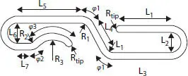
Figure 2.3 Parameterized carcass profile.
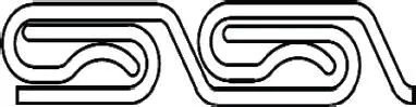
Figure 2.4 Full carcass cross section imported.
Table 2.1 Interlocked carcass cross-section parameters.
| L 1[mm] | 8. 00 | R 1[mm] | 1.00 |
| L 2[mm] | 3. 00 | R 2[mm] | 1.00 |
| L 3[mm] | 9. 00 | R 3[mm] | 3.00 |
| L 4[mm] | 4. 50 | R tip[mm] | 0.50 |
| L 5[mm] | 10. 00 | f 1[°] | 60 |
| L 6[mm] | 3. 00 | f 2[°] | 45 |
| L 7[mm] | 2. 00 | f 3[°] | 90 |
Table 2.2 Interlocked carcass parameters.
| n | 1 |
| K | 1 |
| E [MPa] | 200,000 |
| sp [MPa] | 600 |
| n | 0.3 |
| L p[mm] | 16.00 |
| R inn[mm] | 76.20 |
| t [mm] | 6.40 |
(2.15) 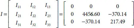
The initial imperfections are given using a helical path that can simulate the initial displacements along both x and y directions using sweep command for two different initial radii that account for ovality equal to L = 0.04. The cross-section is imported in the xz plane and follows half of the elliptical path. The greater diameter is considered along the y direction, instead the other lays on the x direction, as it is shown in Figure 2.5.
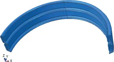
Figure 2.5 Carcass model geometry.
Due to the complex shape, proper of the geometry of the carcass and many possibilities of contact, “General contact” is chosen to simulate the interactions among the three parts, until the buckling collapse is reached. For this unbonded condition, “Frictionless” tangential behavior and “Hard contact” normal behavior with “Allow separation after contact” are chosen. The latter is defined by ( p - h )model, which relates p : contact pressure among surfaces and h : overclosure between contact surfaces respectively. When h < 0, it means no contact pressure, while for any positive contact h is set equal to zero [6].
Also, the plastic behavior of the material is taken into account to verify if the collapse happens in elastic or plastic field and if the hypothesis of considering only elastic behavior in the theoretical model makes sense. As it is shown in Figure 2.6, the material properties for the carcass layer consider a linear elastic behavior, following the Hooke’s law during the first stage then again, a linear behavior due to the plastic tangent modulus for simulating high strain against low stress increments in the plastic field, which accounts for an isotropic hardening law [7].
The external pressure is considered as constant along the width, in z direction and applied directly on the external surface. The kinematic is governed by the boundary conditions that must mainly avoid rigid body displacements. The possibility of assigning symmetric boundary condition with respect to the xz plane is exploited in order to allow displacement in x direction (U1) at the bases of the ring, which also fix the pitch as constant during the simulation. For simulating the occurrence of the local bucking of the ring, the only allowed displacements in the middle of the ring are in y direction (U2), as depicted in Figure 2.7.
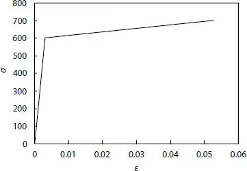
Figure 2.6 Steel strain-stress relationship.
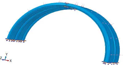
Figure 2.7 Load and boundary conditions.
A dynamic implicit analysis is employed because of the necessity of capture the variation of the stiffness changes step by step in case of non-linearity due to frictionless contact. Non-linear geometry is also taken into account in order to simulate large deformations proper of collapse issue. The dynamic analysis developed, is justified by the fact that the ratio between kinetic energy (ALLKE) and strain energy (ALLSE) for the whole model is kept below 0.1 until the collapse point, in Figure 2.8kinetic and strain energies are plotted against the dimensionless load.
In this model, C3D8R (eight-node continuum linear brick elements with reduced integration and hourglass control) is used for the three parts as can be seen in Figure 2.9. This type of components matches very good the purpose of the model, in fact these can be used for linear and complex non-linear analysis producing high accuracy results when contacts, plasticity and non-linear geometry are considered [8].
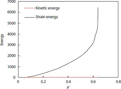
Figure 2.8 ALLKE/ALLSE versus dimensionless load.
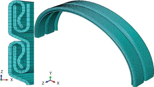
Figure 2.9 Carcass model mesh details, cross-section, and surfaces.
2.3 Comparison and Discussion
The input data for the design case of a flexible pipeline is the internal diameter which is the same for both steel strip reinforced thermoplastic pipes and the case improved against external pressure with stainless steel carcass. For both numerical and numerical models, the chosen reference surface is the outermost and both displacement along x and y directions are analyzed. For the numerical simulation, the central body is chosen as reference, being the only full profile in the model. For the numerical case, displacements could differ one to the other because it simulates the actual geometry as it is shown in Figures 2.10and 2.11While for some theoretical limits, they will be coincident in both directions. By simulating the mechanical behavior of the structure, it is possible to catch the buckling pressure.
Firstly, using the parameters listed in Eq. (2.14)for Eq. (2.10), it is possible to carry out the smallest moment of inertia of the cross-section: I2’ = 185. 41 mm 4. Then, from Eq. (2.9), the equivalent stiffness per unit length is calculated EIeq = 2,317,671.93 MPa mm 3if the mean radius is computed as follows: R = R inn+ t = 79.40 mm. Finally, the critical buckling pressure for a ring without ovality is obtained and it is equal to: pcr = 13.89 MPa. This result is normalized by the critical load at L = 0.04 as shown in Eq. (2.11), and it is plotted in Figure 2.14, which shows the sudden collapse when the structure reaches the collapse pressure.
Читать дальшеИнтервал:
Закладка:
Похожие книги на «Deepwater Flexible Risers and Pipelines»
Представляем Вашему вниманию похожие книги на «Deepwater Flexible Risers and Pipelines» списком для выбора. Мы отобрали схожую по названию и смыслу литературу в надежде предоставить читателям больше вариантов отыскать новые, интересные, ещё непрочитанные произведения.


Обсуждение, отзывы о книге «Deepwater Flexible Risers and Pipelines» и просто собственные мнения читателей. Оставьте ваши комментарии, напишите, что Вы думаете о произведении, его смысле или главных героях. Укажите что конкретно понравилось, а что нет, и почему Вы так считаете.