Omid Bozorg-Haddad - A Handbook on Multi-Attribute Decision-Making Methods

3 (3) The anticipated value or performance of the alternatives with regard to each given criterion. Let v(i,j) represent the value of the ith alternative with respect to the jth criterion, then a m × n matrix is constructed with v(i,j) as the elements; and

4 (4) The decision‐maker prioritizes based on the weights, denoted by {wj | j = 1, 2, …, n}. Each wj reflects the importance of the ith criterion. This step involves a weighting procedure.

Consequently, the decision‐matrix ( D ) is represented as follows (Yu 1990):

(2.1)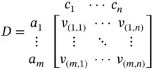

In addition to the decision‐matrix on occasion, the decision‐makers define extreme alternatives, namely, ideal ( a +) and inferior ( a −) alternatives. The ideal alternative is an arbitrarily defined vector of choices describing the aspired solution to the given problem, which, in practice, may or may not be achievable. The inferior alternative is a solution that represents the most undesirable option for the given MADM problem. There are two main methods to compose the ideal and inferior alternatives. One can use the best and worst values in the j th column of the decision‐matrix to compose the j th component of the ideal and inferior alternatives, respectively. On the other hand, one could also use the upper and lower boundaries of the feasible range of the j th criterion to compose these arbitrarily defined alternatives. In such cases, if the criterion is considered to be positive, where the larger the value the better the situation, the upper and lower boundaries represent the ideal and inferior alternatives, respectively. Conversely, a negative criterion, where the smaller the value, the better the situation, the lower and upper boundaries represent the ideal and inferior alternatives, respectively. These arbitrarily defined alternatives can then be represented as follows (Tzeng and Huang 2011):

(2.2)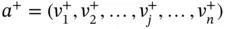

(2.3)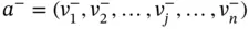

in which and = the components of the ideal and inferior alternatives with regard to the j th criterion, respectively.

The admissibility of each alternative in a MADM problem hinges on their performances with regards to the predefined evaluation criteria, which may be of different mathematical nature. In fact, an MADM problem commonly involves multiple criteria with different dimensions and measure of scales. One of the main challenges of the MADM is for the decision‐maker to aggregate the performance of alternatives with regard to each given criterion so that the overall preference of alternatives can be achieved. However, the former cannot be achieved while the evaluation criteria are not of the same dimension, measuring unit, and scale. Consequently, through a mathematical procedure, better known as normalization, the decision‐matrix is transformed into a dimensionless matrix. There are various normalization procedures, such as the Z ‐score transformation; yet, the following two forms are the most recommended for MADM problems, mainly, because they are easy to interpret (Ebert and Welsch 2004; Zhou et al. 2006; Tzeng and Huang 2011):

Form I: This normalization process, linearly, transforms all the performance values, so that the relative order of magnitude of the ratings remains equal. The procedure can be set up as follows (Chang and Yeh 2001):

For positive criteria: (2.4)

For negative criteria:(2.5)

in which r (i,j)= the normalized performance value for the i th alternatives with respect to the j th criterion.

Form II: In this normalizing procedure, which is slightly more advanced than the former technique, both ideal and inferior alternatives are used to normalize the performance values, as follows (Ma et al. 1999):

For positive criteria:(2.6)

For negative criteria: (2.7)

The cited normalization procedure yields dimensionless performance values of the decision‐matrix in which the [ r (i,j)] range between 0 and 1.

Through the normalization procedure, the decision‐maker transforms the elements of a decision‐matrix into commensurable values. The next step is for the decision‐maker to combine these values in a way that the alternatives’ overall preferences can be evaluated. Herein, assume that the decision‐maker evaluated the importance of each criterion and derive the set of weights that best reflect the stakeholder’s priorities. Let w jdenote the assigned weight to the j th criterion; the following holds for the assigned weight set:

(2.8)

Assigning the proper weight to each criterion is a challenging procedure that is discussed later in the appendix section. The challenge remains, however, on how these values can be combined to form an overall preference for each given alternative. Sections 2.2and 2.3describe, in detail, two basic methods to aggregate the alternatives’ performances and obtain the alternatives’ overall preference.

The weighted sum method (WSM), also referred to as the simple additive weighting (SAW) method, is the best known and simplest MADM method for evaluating a number of alternatives in terms of a number of decision criteria. The basic logic of WSM, which was perhaps the first logical solution that enabled the decision‐makers to cope with the MADM problems, is to obtain a weighted sum of the performance values of each alternative's overall attributes. Churchman and Ackoff (1954) were among the first to employ the WSM method to cope with a portfolio selection problem (Tzeng and Huang 2011). Ever since, due to the simplistic nature of the method, it quickly became a popular tool to cope with a MADM problem (Zanakis et al. 1995, 1998). Notable examples of applying WSM in different fields would be in agroecosystem management (Andrews and Carroll 2001), airlines' strategic planning and management (Chang and Yeh 2001), energy planning and management (San Cristóbal 2011), construction management (Jato‐Espino et al. 2014), environmental assessments (Kang 2002; Zhou et al. 2006), forestry management (Howard 1991), industrial management (Ma et al. 1999), industrial robot selection (Athawale and Chakraborty 2011), landfill site selection (Şener et al. 2006), mobile network selection (Savitha and Chandrasekar 2011), software evaluation (Olson et al. 1995), wastewater management (Zarghami 2011), and water supply planning (Goicoechea et al. 1992; Hobbs et al. 1992), to name a few.

The following is a detailed stepwise instruction to implement WSM as an MADM solving method:

The initial step of the WSM would be for the decision‐maker to determine the elements of the decision‐matrix. It goes without saying that the integrity of the final result would rely heavily on this step. A well‐defined decision‐matrix is the basic requirement of any MADM method.