Space Physics and Aeronomy, Ionosphere Dynamics and Applications

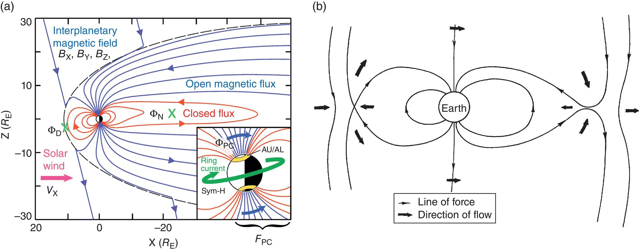
Figure 2.2 (a) A schematic of the magnetosphere showing closed (red) and open (blue) magnetic field lines. Green crosses mark the approximate locations of magnetopause and magnetotail reconnection X‐lines for southward IMF. The inset panel shows the relationship between closed field lines and the auroral zone, and open field lines and the polar cap (after Milan et al., 2009). (b) The Dungey cycle of magnetospheric convection. Arrowed lines are magnetic field lines in the solar wind (left and right) and of the magnetosphere (joined to the Earth). Magnetic reconnection occurs in front of and behind the Earth. Arrows show the sense of plasma flow, mainly antisunward, though with sunward flow within the magnetosphere

(from Milan (2009): https://www.ann‐geophys.net/27/659/2009/. Licensed under CC BY 3.0; from Dungey, 1961: Reproduced with permission of American Physical Society).

Field lines colored red in Figure 2.2a, known as “closed” field lines, have both ends on the surface of the Earth. Blue field lines are “open,” interlinking with the interplanetary medium. As first speculated by Dungey (1961, 1963), at interfaces in the plasma where there is a strong shear in the magnetic field, such as at the subsolar magnetopause when IMF B Z< 0 (dayside green cross), “magnetic reconnection” can take place to link the otherwise segregated regions. In Figure 2.2a, IMF field lines are shown that have undergone reconnection with closed field lines at the magnetopause and are in the process of being carried antisunward by the flow of the solar wind to form the “magnetotail.” The open field lines of the tail are known as the “magnetotail lobes.” The erosion of the dayside magnetosphere by reconnection cannot continue indefinitely: eventually magnetic reconnection is initiated between the oppositely directed field lines in the central plane of the magnetotail, the “neutral sheet,” to reclose flux (nightside green cross). As indicated in Figure 2.2b, the opening and closing of flux leads to an antisunward motion of flux and plasma across the high‐latitude regions of the magnetosphere and sunward return flow at low latitudes, known as the “Dungey cycle” (Dungey, 1961).

After reconnection has taken place at the magnetopause, protons and electrons from the solar wind can enter the magnetosphere by moving along the newly opened field lines and across the magnetopause. The volume of the lobes is large, so the plasma is tenuous here (~0.01 cm −3). However, as the field lines convect toward the neutral sheet, the plasma is heated and compressed to a density of ~1 cm −3to form the “plasma sheet,” roughly coincident with the closed field line regions of Figure 2.2a. The hot plasma at the inner edge of the plasma sheet encircles the Earth forming an electric current system known as the “ring current.”

The inset of Figure 2.2a shows where the magnetospheric field lines have their footprints in the ionosphere, poleward of approximately 60 olatitude. The closed field line region and plasma sheet maps to the “auroral zones,” where the majority of auroras are produced. The open field lines of the lobes map to the regions poleward of the auroral zones, known as the “polar caps,” which are largely devoid of auroras. Magnetospheric convection is communicated to the polar ionosphere, and constitutes the high‐latitude convection that is the focus of this review. Closed field lines equatorward of the auroral zones map to the “plasmasphere,” a region of cold, dense (~10–1,000 cm −3) plasma of ionospheric origin, which corotates with the planet. In this low‐latitude region, the ionosphere is approximately stationary with respect to the Earth's surface, neglecting solar‐quiet convection and the equatorial fountain.

The ionosphere is the lower boundary of the magnetosphere, where plasma and neutral particles intermingle. The ionosphere is produced by ionization of the upper atmosphere, predominantly by extreme ultraviolet (EUV) photons from the Sun, and the impact of energetic charged particles precipitating from the magnetosphere. The geographical distribution and altitude profile of ionization is determined by competition between the source and loss processes, described by Chapman theory in the case of solar illumination (Chapman, 1931) as well as transport. On the dayside of the planet, this results in an altitude profile that comprises three layers or regions: the F region, with a peak free‐electron concentration or density of 10 11to 10 12m −3near an altitude of 300 km; the E region of 10 10to 10 11m −3at 110 km; and the D region of 10 8m −3at 90 km. In the F region, the density of the neutral atmosphere is sufficiently low that recombination is slow, such that the F region density can persist for many tens of minutes even if the source is removed; at E and D region altitudes, recombination is rapid and these layers disappear almost immediately. On the nightside of the Earth, the ionosphere is depleted owing to the lack of photoionization. Residual ionization occurs in the F region to the east of the dusk terminator as recombination is slow. In addition, transport of high concentration plasma from the dayside within the polar convection pattern can maintain F region ionization in sporadic patches in the dark polar caps. Impact ionization associated with auroral processes leads to elevated D, E, and F region densities in the auroral zones. Figure 2.3b shows in schematic form the approximate location of elevated ionospheric density (grey shading) relative to the twin‐cell convection pattern. The position of the solar terminator changes with season and time of day.

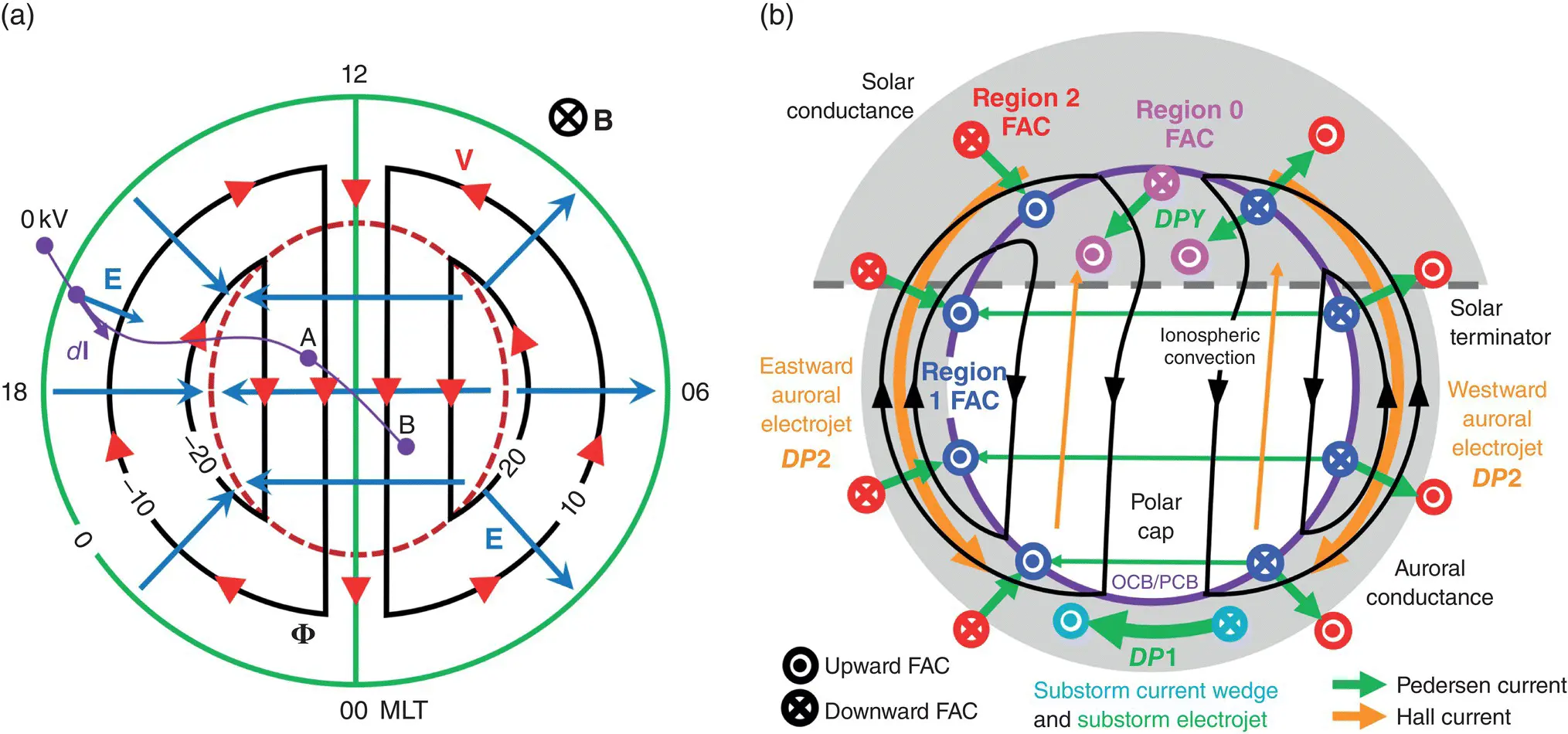
Figure 2.3 (a) The relationship between ionospheric flow, electric field, and electrostatic potential. The magnetic field points everywhere into the page. The green circle represents the low‐latitude boundary of the ionospheric convection, also the zero potential contour. Red arrows indicate directions of ionospheric flow, with the associated electric field distribution shown in blue. The potential Φ at a point A or B is determined by integrating − E∙ d lfrom a point of zero potential along any path (e.g., purple line) to that location. Contours of potential (or equipotentials) are shown by the black curves, at potential steps of 10 kV. The voltage between two points A and B is the integral of − E∙ d lbetween them, also given by Φ B− Φ A. The red dashed line shows the polar cap boundary. (b) The association of ionospheric current systems and FACs with the convection pattern

(from Milan et al., 2017; Reproduced with permission of Springer Nature).

The ionosphere is a magnetized plasma, comprising free charge carriers suffused by the Earth's dipolar magnetic field. Hence, electric and magnetic forces play an important role in determining the dynamics and structure of the ionosphere and its interaction with the magnetosphere and solar wind. The next section introduces the basic plasma physics necessary to understand the magnetosphere‐ionosphere coupled system.

A charged particle of mass m and charge q moving with velocity vin the presence of an electric field Eand magnetic field B, experiences the Lorentz force