Michael Graham - Wind Energy Handbook

Blade solidity σ is defined as total blade area divided by the rotor disc area and is a primary parameter in determining rotor performance. Chord solidity σ ris defined as the total blade chord length at a given radius divided by the circumferential length around the annulus at that radius:

(3.56)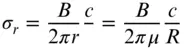

It is argued by Wilson et al. (1974) that the drag coefficient should not be included in Eqs. (3.54aor b) and (3.55)because the velocity deficit caused by drag is confined to the narrow wake that flows from the trailing edge of the aerofoil. Furthermore, Wilson and Lissaman reason, the drag based velocity deficit is only a feature of the wake and does not contribute to the velocity deficit upstream of the rotor disc. The basis of the argument for excluding drag in the determination of the flow induction factors is that, for attached flow, drag is caused only by skin friction and does not affect the pressure drop across the rotor. Clearly, in stalled flow the drag is overwhelmingly caused by pressure. In attached flow – see, e.g. Young and Squire (1938) – the modification to the inviscid pressure distribution around an aerofoil caused by the boundary layer has a small effect both on lift and drag. The ratio of pressure drag to total drag at zero angle of attack is approximately the same as the thickness to chord ratio of the aerofoil and increases as the angle of attack increases.

One last point about the BEM theory: the theory neglects the axial components of the pressure forces at curved boundaries between streamtubes. It is more accurate if the blades have uniform circulation, i.e. if a is uniform. For non‐uniform circulation there is increased radial interaction and exchange of momentum as a result of normal pressure and viscous shear forces between flows through adjacent elemental annular streamtubes. However, in practice, it appears that the error involved is small for tip speed ratios greater than three.

The calculation of torque and power developed by a rotor requires a knowledge of the flow induction factors, which are obtained by solving Eqs. (3.54aor b) and (3.55). The solution is usually carried out iteratively because the 2‐D aerofoil characteristics are non‐linear functions of the angle of attack.

To determine the complete performance characteristic of a rotor, that is, the manner in which the power coefficient varies over a wide range of tip speed ratio, requires the iterative solution.

The iterative procedure is to assume a and a ′to be zero initially, determining ϕ , C l, and C don that basis, and then to calculate new values of the flow factors using Eqs. (3.54aor b) and (3.55). The iteration is repeated until convergence is achieved.

From Eq. (3.49), the torque developed by the blade elements of spanwise length δr is

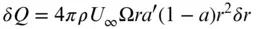
If drag, or part of the drag, has been excluded from the determination of the flow induction factors, then its effect must be introduced when the torque is calculated [see Eq. (3.49)]:

The complete rotor, therefore, develops a total torque Q :

(3.57)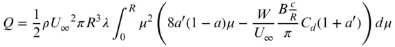

The power developed by the rotor is P = Q Ω

The power coefficient is, therefore,

Solving the blade element − momentum Eqs. (3.54aor b) and (3.55)for a given, suitable blade geometrical and aerodynamic design yields a series of values for the power and torque coefficients that are functions of the tip speed ratio. A typical performance curve for a modern, high‐speed wind turbine is shown in Figure 3.15.

The maximum power coefficient occurs at a tip speed ratio for which the axial flow induction factor a , which in general varies with radius, approximates most closely to the Betz limit value of . At lower tip speed ratios the axial flow induction factor can be much less than and aerofoil angles of attack are high, leading to stalled conditions. For most wind turbines stalling is more likely to occur at the blade root because, from practical constraints, the pitch angle β due to built‐in twist of a blade is not large enough in that region. At low tip speed ratios blade stalling is the cause of a significant loss of power, as demonstrated in Figure 3.15. At high tip speed ratios a is high, angles of attack are low, and drag begins to predominate. At both high and low tip speed ratios, therefore, drag is high and the general level of a is non‐optimum so the power coefficient is low. Clearly, it would be best if a turbine can be operated at all wind speeds at a tip speed ratio close to that which gives the maximum power coefficient.

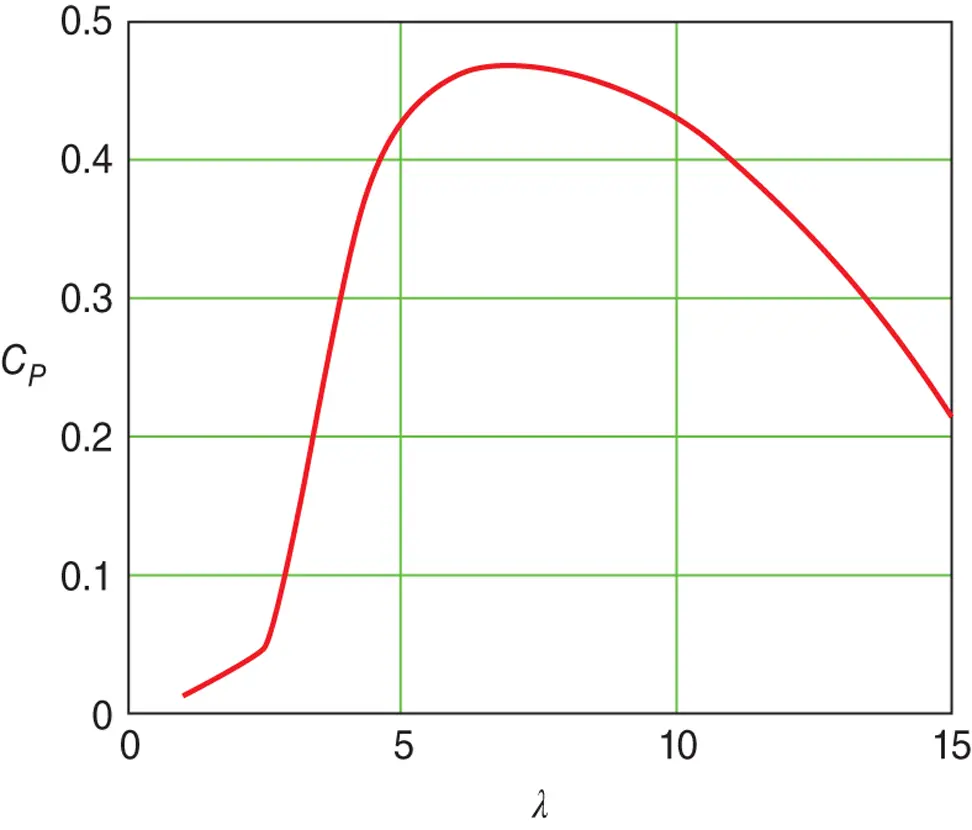
Figure 3.15 Power coefficient – tip speed ratio performance curve.

Actuator line theory combines the 2‐D blade sectional characteristics used in BEM theory with, usually, a CFD grid calculation of the whole flow field external to the rotor blades including the wake. It is particularly useful for calculating the aerodynamic loads and flow field quantities where wind turbine rotors operate within a larger complex flow field such as a wind farm or a non‐simple ABL topography.

In this method, the outer flow is computed on a finite volume or element grid by some method of numerical simulation (usually viscous and turbulent) of the unsteady flow equations, such as unsteady Reynolds averaged Navier–Stokes (URANS) or LES (see discussion in Chapter 4). A number of open‐source or commercial codes are available to do this with varying degrees of fidelity and cost. Because the computations are carried out over a sequence of timesteps and are spatially 3‐D, this always requires significant computing resource. The discretisation scale should be appropriate to resolve the major structures of the ABL and its turbulence and the rotor (diameters) and the turbulent structures in their wakes. But it does not resolve the flows on the length scales of the blade chords and their boundary layers and hence is orders of magnitude faster than a complete simulation of all scales in the flow field.

Instead of resolving the sectional blade flows, these are replaced, as in BEM theory, by aerofoil characteristics from look‐up tables (or possibly a fast panel method such as XFOIL; Drela 1989). The rotor blades are tracked through the outer flow grid and the velocity field, which has been computed on that grid, is interpolated onto the designated rotor blade sections. The resulting sectional blade forces obtained by interpolating from the blade characteristic look‐up tables are projected back onto the outer grid as a series of momentum sinks for the components of force in the three coordinate directions. These sinks then form part of the grid flow field calculation at the next timestep. This coupling between the inner and outer flow calculations may be either loose going from timestep to timestep as indicated or may be a strong coupling in which the flow is converged within each timestep by iteration or by solving the whole in a single very large matrix. Transfer of force and large‐scale velocities between the inner and outer flow fields is well established, but methods of determining the effective turbulence input from the smaller‐scale structures in the rotor blade flows as sources for the larger‐scale outer flow are not, and further work is required here. Good references for this method are Mikkelsen (2003) and Troldborg et al. (2006).