Anand K. Verma - Introduction To Modern Planar Transmission Lines

(4.3.14)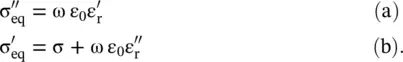

Sometimes, loss due to the polarization causing is ignored, say in a semiconductor, if the loss due to the conduction current is more significant. The loss characteristic of a semiconducting substrate is given by its conductivity. In that case, the loss‐tangent is expressed in terms of the conductivity of a medium:

(4.3.15)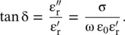

The above expression helps to convert the conductivity of a substrate to its loss‐tangent at each frequency of the required frequency band. It can also be used to convert the loss‐tangent to the conductivity at each frequency.

The equivalence between the relative permittivity and capacitance has been obtained by treating both the dielectric and capacitor as electric energy storage devices. Thus, the complex relative permittivity is equivalent to a complex capacitance. Figure (4.6b)provides the admittance of a lossy capacitor:

(4.3.16)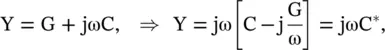

where the complex capacitance C *is given by

(4.3.17)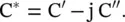

The real and imaginary parts of a complex capacitance, and also loss‐tangent, are given by the following expressions:

(4.3.18)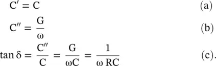

The complex relative permittivity is also expressed as follows:

(4.3.19)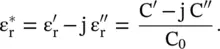

The above expression is helpful in the computation of the real and imaginary parts of the effective relative permittivity of a lossy planar transmission line. The complex line capacitance of a lossy planar transmission line can be numerically evaluated. It also helps to compute the effective loss‐tangent of a multilayered planar transmission line by the variational method . It is discussed in chapter 14.

The magnetic loss in magnetic materials is due to the process of magnetization that results in a complex relative permeability, . The relative permeability is defined as a ratio of two inductances; inductance (L *) of the coil with a magnetic material, and inductance (L 0) of the same coil with the air‐core,

(4.3.20)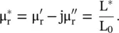

A magnetic material placed inside a coil, shown in Fig. (4.7a), gets magnetized in the process of magnetization . The current causing the magnetization is known as the magnetization current (I m). However, during the magnetization process, some power is lost. It is viewed through the magnetic loss‐current (I r). The magnetization of a magnetic material involves the storage of magnetic energy. So, a lossy magnetic material is modeled through the RL equivalent circuit, shown in Fig. (4.7b). The inductor models the stored magnetic energy in a magnetic material, whereas the resistor models its loss.

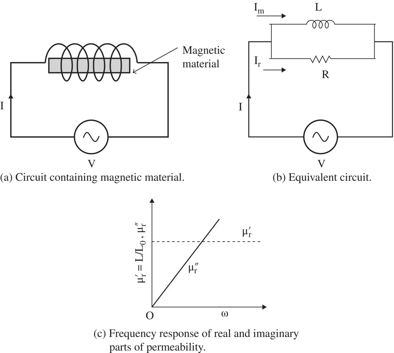
Figure 4.7 Circuit model and frequency response of lossy magnetic material.

A time‐harmonic current I = I 0e jωtflows through the coil containing the magnetic material. The voltage across the coil and current through it are given below:

(4.3.21)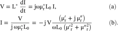

Figure (4.7b)shows the current flowing in the parallel RL equivalent circuit. By comparing the above current, with the circuit model current; the expressions for the circuit elements, in terms of the material parameters, are obtained as follows:

(4.3.22)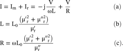

The magnetic loss‐tangent of the lossy inductor is defined below that helps to get the magnetic loss‐tangent of magnetic material:

(4.3.23)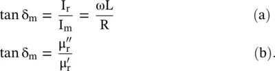

A lossless magnetic material has , i.e. , R → ∞. It means an inductor, without the resistor, models the lossless magnetic material. It shows that the permeability is an ability of a magnetic material to store magnetic energy, just as the permittivity of dielectric material is its ability to store electric energy . For the case of the low‐loss magnetic materials, , the following expressions are obtained from equations (4.3.22b)and (4.3.22c):

(4.3.24)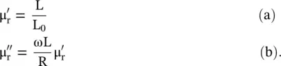

It is observed that for a low‐loss magnetic material, is independent of frequency, whereas increases linearly with frequency, as shown in Fig. (4.7c). The above equations show that inductor models the real part of the complex permeability, whereas resistance models its imaginary part . This kind of frequency response may not be a realistic description of a hysteretic magnetic material.

The experimental observations on the time‐dependent electromagnetic field are described by a set of the vector differential equations, known as the Maxwell equations. These sets of equations form the fundamental laws of nature, governing behaviors of the EM‐field in free space, and also in material media. Each part of Maxwell equations shows a definite nature of the EM‐field, explored by different investigators; Faraday, Ampere, and Gauss. However, Maxwell has put them in the form of a consistent set of equations using a mathematical format called the quaternions . He has also introduced the concept of displacement current . On solving the equations, either for the electric field or the magnetic field, the wave equations are obtained for the electric and magnetic fields traveling at a velocity of light in free space. Poynting has determined the power carried by the EM‐wave. Finally, Heaviside replaced the quaternions by the vector notations and presented the Maxwell equations in the present form, i.e. in the convenient form of the vector differential equations [B.26–B.28]. Such a formulation of the electromagnetic theory has opened the grand path of modern research and investigation. So, the modern form of Maxwell equations can be truly called Maxwell–Heaviside equations . However, in this text, we use normal terminology to follow the current practice.