Anand K. Verma - Introduction To Modern Planar Transmission Lines

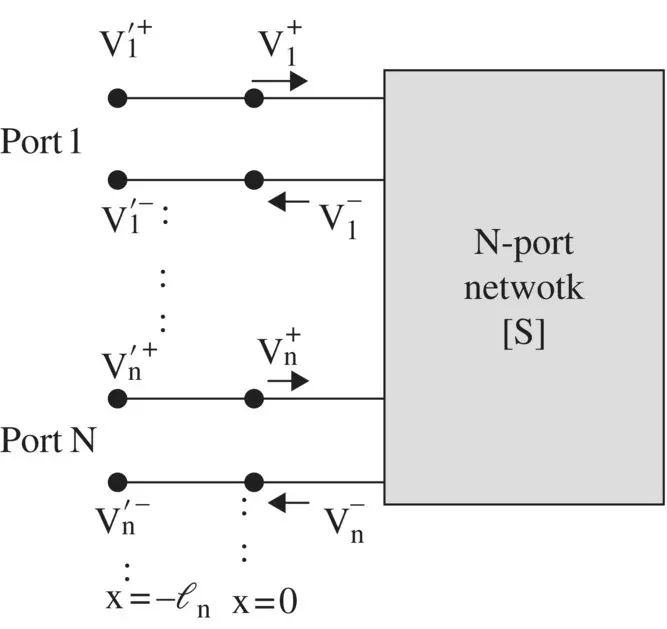
Figure 3.13 N‐port network showing phase‐shifting property.

For an N‐port network, the incident wave at the n thport, x = − ℓ n, after reflection from the port at x = 0, returns to x = − ℓ n. In the process, it travels the electrical length 2θ n. Similarly, if the wave is incident at port #1, located at x = − ℓ 1and arrives at the port‐2, located at x = − ℓ 2; the electrical length traveled by the wave is θ 1+ θ 2= β 1ℓ 1+ β 2ℓ 2, or 2θ 1, on the assumption that β 1= β 2, and ℓ 1= ℓ 2, i.e. the transmission lines connected at both the ports are identical. The measured or simulated scattering matrix [S ′] at the location x = − ℓ nis related to the [S] parameters of the network by the following expression

(3.1.54)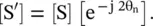

The [S]‐parameter of the network is extracted from equation (3.1.54), as

(3.1.55)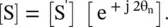

For reducing the cascaded network to a single equivalent network, the [S] parameters cannot be cascaded like the [ABCD] parameters. The [ABCD] matrix is suitable for this purpose. However, it is not defined in terms of the power variables. Therefore, another suitable transmission matrix, called [T] matrix has been defined in terms of the power variables to cascade the microwave networks. The [S] matrix is easily converted to the [T] parameters [B.1, B.2–B.5, B.7, B.9].

The concept of the [S] matrix is used below to some simple, but useful circuits. These examples would help to appreciate the applications of the [S] parameters.

Determine the S‐parameters and return loss of a 2‐port network with arbitrary termination shown in Fig (3.14).

The 2‐port network (device) is connected to a source at the port‐1 and a load Z Lat the port‐2. The source has voltage V gwith internal impedance Z g. The network scattering parameters‐[S] are computed under the matched condition. The characteristic impedance of the connecting line between the port‐1 and the source is Z 01, whereas the characteristic impedance of the connecting line between the port‐2 and the load is Z 02. The lengths of the connecting lines are zero. The reflection and transmission coefficients are to be determined at the input and output terminals. This is a practical problem for the measurement and simulation of the 2‐port network:

(i)

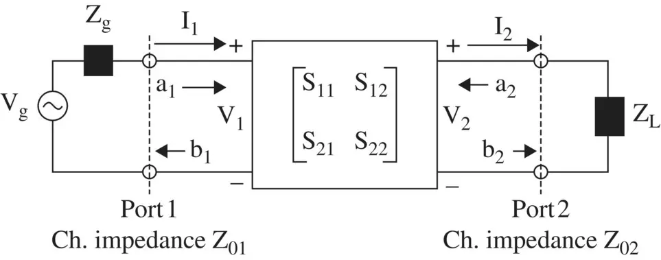
Figure 3.14 A two‐port network with arbitrary termination.

Figure (3.14)shows that the power variable b 2is the incident wave at the load Z Land the power variable a 2is the reflected wave from the load. Thus, the reflection coefficient at the load is

(ii)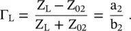

From above equations (i)and (ii):

(iii)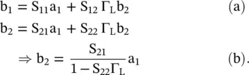

On substituting b 2from equation (b) in equation (a):

(iv)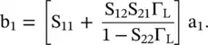

The input reflection coefficient at the port‐1 is

(3.1.56)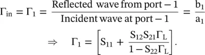

The reflection coefficient Γ 1is more than S 11of the network. The mismatch at the load degrades the return loss (RL) of the network. It is given by

(3.1.57)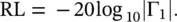

For the port 2 open‐circuited (Z L→ ∞), the waves get reflected in‐phase, i.e. Γ L= 1, and for a short‐circuited load (Z L= 0) the total reflection is out of phase, i.e. Γ L= −1. If the network is terminated in a matched load (Z L= Z 02), the incident waves are absorbed with Γ L= 0 and Γ 1= S 11. Likewise, the source reflection coefficient Γ gcould be defined at the input port‐1. Figure (3.14)again shows that b 1is the incident wave on the internal impedance of the source Z gand a 1is the reflected wave from Z g.Thus,

(v)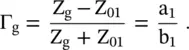

The output reflection coefficient Γ 2at the port‐2 is obtained from equations (i)and (v):

(3.1.58)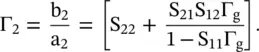

Again under the matched condition (Z g= Z 01) at the input port, Γ g= 0. For most of the applications, 50 Ω system impedance is used, i.e. Z 01= Z 02= Z 0= 50 Ω. For a 2‐port lossless network, we have the following expressions:

However, for a reciprocal network S 12= S 21. Thus, the above equations provide

(3.1.59)

The network also follows 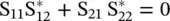. The S‐parameters are complex quantities. The S‐parameters are written in the phasor form: 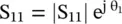, 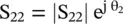and S 12= |S 12| e j ϕ. From the above equation, the phase relation is obtained:

(3.1.60)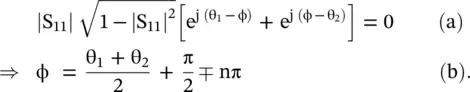

Therefore, once the complex S 11and S 22are measured, both the magnitude and phase of the S 21are determined. However, usually, both S 11and S 21are obtained from a VNA and also from the circuit simulator or EM‐simulator. The magnitude of S 21provides the insertion‐loss of the network and ϕ is the phase shift at the output of the network.