Anand K. Verma - Introduction To Modern Planar Transmission Lines

The reflection coefficient at the j thport is obtained from equation (3.1.40):

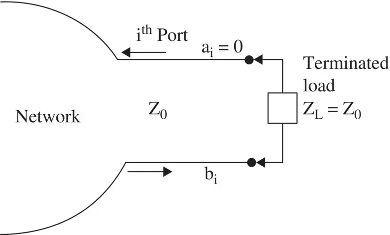
Figure 3.12 At the i thport, the load is terminated in port characteristic impedance.

(3.1.41)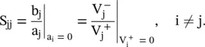

Therefore, S jjis the reflection coefficient (Γ j) at the j thport, provided all other ports are terminated in their characteristic impedances. However, if other ports are not terminated in their characteristic impedances, then S jjis not a measure of the true reflection coefficient of the network or a device at the j thport. The true reflection coefficient at the j thport, under the unmatched load condition, is more than S jjthat is defined under the matched load condition.

If the excitation source is connected only to the j thport and the response is seen at the i thport, while all other ports are terminated in their characteristic impedances, it leads to . It shows that the excitation is zero at all ports, except at the j thport. The transmitted power, i.e. the scattered power, from the j thport is available at all ports, i = 1, 2, …, k. However, at the j thport, a part of the incident power appears as the reflected power. The transmission coefficient , S ijfor the power transfer from the j thport to the i thport is defined as

(3.1.42)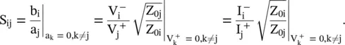

Normally, the network has identical port impedances and equal to the system impedance, i.e. Z 0i= Z 0j= Z 0. Equation (3.1.40)is written in compact form as

(3.1.43)

The elements of the [S] matrix are determined using equations (3.1.41)and (3.1.42).

Some important properties of the [S] matrix description of the network are summarized below, without going for the formal proof of these statements. Usually, elements of the [S] matrix are complex quantities. The detailed discussion is available in the well‐known textbooks [B.1–B.5, B.7].

The [S] matrix of a reciprocal network is a symmetric matrix, i.e. the transpose [S] Tof the [S] matrix is equal to the [S] matrix itself:

(3.1.44)

The [S] matrix of a lossless network is a unitary one. However, if the network is not lossless, then it is not unitary. The definition of the unitary matrix provides the following relation for the given [S] matrix:

(3.1.45)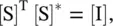

where [S] Tis the transpose of the [S] matrix, [S] *is a complex conjugate of the complex [S] matrix and [I] is the identity matrix. Thus, for a given 2‐port [S] matrix, we have

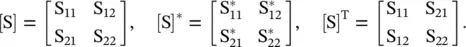
On substituting these expressions in the unitary relation (3.1.45), the following result is obtained:

(3.1.46)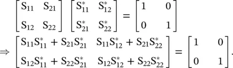

On equating each element of matrix equation (3.1.46), the following relations are obtained:

(3.1.47)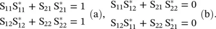

Equations (3.1.47)are generalized for the N‐port network:

(3.1.48)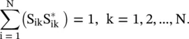

(3.1.49)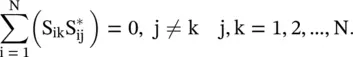

Equation (3.1.48)shows that both elements have identical columns, whereas in equation (3.1.49)column are not identical. The [S] matrix is formed by the column vector as follows:

(3.1.50)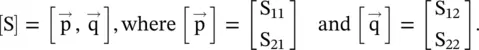

Therefore, in the usual vector notation we have

(3.1.51)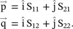

Hence, for a lossless network the following statements, based on equations (3.1.48)and (3.1.49)are made:

The dot product of any column vector with its complex conjugate is unity,

The dot product of any column vector with the complex conjugate of any other column vector is zero,

The [S] matrix forms an orthogonal set of the vectors.

The following expressions are written from equation (3.1.47):

(3.1.52)

Equation (3.1.52)is the power balance equations for the lossless two‐port networks. The unit input power fed to the port‐1 is a sum of the reflected power ( |S 11| 2) at the port‐1 and the transmitted power |S 21| 2to the port‐2. In the case |S 11| 2+ |S 21| 2is less than unity, some power is lost in the network through the mechanism of conductor, dielectric, and radiation losses. The lost power, i.e. the power dissipation in the network, is

(3.1.53)

The [S] parameter is a complex quantity. It has both magnitude and phase. Thus, the [S]‐parameter is always defined with respect to a reference plane . In Fig (3.13)[S]‐parameter of the N‐port network is known at the location x = 0. It is determined at the new location, x = −ℓ n. Alternatively, once the [S] parameters are known at x = −ℓ n, these are determined at x = 0, i.e. at the port of the network. The location ℓ nshows the length of the line connected to each port of an N‐port network. Normally, it is the point of measurement of the [S] parameters of the network or device. The interconnecting transmission line is lossless and has propagation constant β n. Thus, the electrical length of the connecting line is θ n= β nℓ n.