Paul A. Gagniuc - Algorithms in Bioinformatics

1 Cover

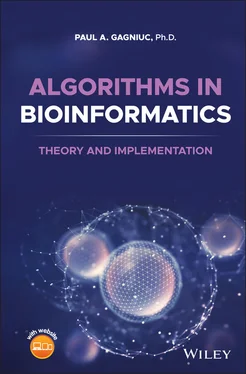
2 Title Page Algorithms in Bioinformatics Theory and Implementation Paul A. Gagniuc University Politehnica of Bucharest Bucharest, Romania

3 Copyright

4 Dedication

5 Preface

6 About the Companion Website

7 1 The Tree of Life (I)1.1 Introduction 1.2 Emergence of Life 1.3 Classifications and Mechanisms 1.4 Chromatin Structure 1.5 Molecular Mechanisms 1.6 Known Species 1.7 Approaches for Compartmentalization 1.8 Sizes in Eukaryotes 1.9 Sizes in Prokaryotes 1.10 Virus Sizes 1.11 The Diffusion Coefficient 1.12 The Origins of Eukaryotic Cells 1.13 Origins of Eukaryotic Multicellularity 1.14 Conclusions

8 2 Tree of Life: Genomes (II)2.1 Introduction 2.2 Rules of Engagement 2.3 Genome Sizes in the Tree of Life 2.4 Organellar Genomes 2.5 Plasmids 2.6 Virus Genomes 2.7 Viroids and Their Implications 2.8 Genes vs. Proteins in the Tree of Life 2.9 Conclusions

9 3 Sequence Alignment (I)3.1 Introduction 3.2 Style and Visualization 3.3 Initialization of the Score Matrix 3.4 Calculation of Scores 3.5 Traceback 3.6 Global Alignment 3.7 Local Alignment 3.8 Alignment Layout 3.9 Local Sequence Alignment – The Final Version 3.10 Complementarity 3.11 Conclusions

10 4 Forced Alignment (II)4.1 Introduction 4.2 Global and Local Sequence Alignment 4.3 Experiments and Discussions 4.4 Advanced Features and Methods 4.5 Conclusions

11 5 Self-Sequence Alignment (I)5.1 Introduction 5.2 True Randomness 5.3 Information and Compression Algorithms 5.4 White Noise and Biological Sequences 5.5 The Mathematical Model 5.6 Noise vs. Redundancy 5.7 Global and Local Information Content 5.8 Signal Sensitivity 5.9 Implementation 5.10 A Complete Scanner for Information Content 5.11 Conclusions

12 6 Frequencies and Percentages (II)6.1 Introduction 6.2 Base Composition 6.3 Percentage of Nucleotide Combinations 6.4 Implementation 6.5 A Frequency Scanner 6.6 Examples of Known Significance 6.7 Observation vs. Expectation 6.8 A Frequency Scanner with a Threshold 6.9 Conclusions

13 7 Objective Digital Stains (III)7.1 Introduction 7.2 Information and Frequency 7.3 The Objective Digital Stain 7.4 Interpretation of ODSs 7.5 The Significance of the Areas in the ODS 7.6 Discussions 7.7 Conclusions

14 8 Detection of Motifs (I)8.1 Introduction 8.2 DNA Motifs 8.3 Major Functions of DNA Motifs 8.4 Conclusions

15 9 Representation of Motifs (II)9.1 Introduction 9.2 The Training Data 9.3 A Visualization Function 9.4 The Alignment Matrix 9.5 Alphabet Detection 9.6 The Position-Specific Scoring Matrix (PSSM) Initialization 9.7 The Position Frequency Matrix (PFM) 9.8 The Position Probability Matrix (PPM) 9.9 The Position Weight Matrix (PWM) 9.10 The Background Model 9.11 The Consensus Sequence 9.12 Mutational Intolerance 9.13 From Motifs to PWMs 9.14 Pseudo-Counts and Negative Infinity 9.15 Conclusions

16 10 The Motif Scanner (III)10.1 Introduction 10.2 Looking for Signals 10.3 A Functional Scanner 10.4 The Meaning of Scores 10.5 Conclusions

17 11 Understanding the Parameters (IV)11.1 Introduction 11.2 Experimentation 11.3 Signal Discrimination 11.4 False-Positive Results 11.5 Sensitivity Adjustments 11.6 Beyond Bioinformatics 11.7 A Scanner That Uses a Known PWM 11.8 Signal Thresholds 11.9 Conclusions

18 12 Dynamic Backgrounds (V)12.1 Introduction 12.2 Toward a Scanner with Two PFMs 12.3 A Scanner with Two PFMs 12.4 Information and Background Frequencies on Score Values 12.5 Dynamic Background vs. Null Model 12.6 Conclusions

19 13 Markov Chains: The Machine (I)13.1 Introduction 13.2 Transition Matrices 13.3 Discrete Probability Detector 13.4 Markov Chains Generators 13.5 Conclusions

20 14 Markov Chains: Log Likelihood (II)14.1 Introduction 14.2 The Log-Likelihood Matrix 14.3 Interpretation and Use of the Log-Likelihood Matrix 14.4 Construction of a Markov Scanner 14.5 A Scanner That Uses a Known LLM 14.6 The Meaning of Scores 14.7 Beyond Bioinformatics 14.8 Conclusions

21 15 Spectral Forecast (I)15.1 Introduction 15.2 The Spectral Forecast Model 15.3 The Spectral Forecast Equation 15.4 The Spectral Forecast Inner Workings 15.5 Implementations 15.6 The Spectral Forecast Model for Predictions 15.7 Conclusions

22 16 Entropy vs. Content (I)16.1 Introduction 16.2 Information Entropy 16.3 Implementation 16.4 Information Content vs. Information Entropy 16.5 Conclusions

23 17 Philosophical Transactions17.1 Introduction 17.2 The Frame of Reference 17.3 Random vs. Pseudo-random 17.4 Random Numbers and Noise 17.5 Determinism and Chaos 17.6 Free Will and Determinism 17.7 Conclusions

24 Appendix A A.1 Association of Numerical Values with Letters A.2 Sorting Values on Columns A.3 The Implementation of a Sequence Logo A.4 Sequence Logos Based on Maximum Values A.5 Using Logarithms to Build Sequence Logos A.6 From a Motif Set to a Sequence Logo

25 References

26 Index

27 End User License Agreement

1 Chapter 1 Table 1.1 The total number of known species. Table 1.2 Extreme sizes of unicellular organisms. Table 1.3 Extreme sizes in viruses. Table 1.4 Single-celled organisms vs. viruses.

2 Chapter 2 Table 2.1 The average genome size in the tree of life. Table 2.2 The average genome size in prokaryotes. Table 2.3 The average genome size in different eukaryotic organelles. Table 2.4 The average DNA length of different plasmids. Table 2.5 The average genome size of different eukaryotic and prokaryotic viruse... Table 2.6 Genes vs. proteins in the tree of life.

3 Chapter 3 Table 3.1 Traceback start and stop locations.

4 Chapter 4Table 4.1 Global alignment and Local alignment.Table 4.2 Examples of alignments and associated scores.Table 4.3 The significance thresholds based on TRNG and MCG .Table 4.4 Forced alignment and local alignment.Table 4.5 RIK examples for one multivalue record from local storage.

5 Chapter 5Table 5.1 An intuitive step-by-step calculation example.Table 5.2 A signal extraction based on local information content.Table 5.3 A convergence test of the local regime for sliding windows of differen...

6 Chapter 6Table 6.1 Additional experiments on frequencies.

7 Chapter 8Table 8.1 Examples of DNA motifs.Table 8.2 Splicing motifs from human genes.

8 Chapter 9Table 9.1 A set of motifs.Table 9.2 Examples of alphabets for different sequences.Table 9.3 The fate of a PPM value.Table 9.4 Sets of variations for null models.Table 9.5 The null model in PPM format.Table 9.6 Motif set vs. consensus.Table 9.7 Examples of pseudo-counts and their effects on the negative scale.

9 Chapter 10Table 10.1 Additional tests by using pseudo-counts.Table 10.2 The meaning of scores.Table 10.3 Range of values for scores.

10 Chapter 11Table 11.1 Scanner discrimination power.Table 11.2 Signal filters and thresholds.

11 Chapter 12Table 12.1 Tests performed with pseudo-counts and two PFMs (real background).Table 12.2 Additions to the background set.Table 12.3 Tests performed on a scanner with two PFMs.Table 12.4 Detection and contrast.Table 12.5 Information content and score values.

12 Chapter 13Table 13.1 Transition matrices and specially constructed sequences .

13 Chapter 14Table 14.1 The meaning of scores.

14 Chapter 15Table 15.1 Results of the two halves of the spectral forecast equation.Table 15.2 Experiments on the spectral forecast equation by using a single matri...Table 15.3 Experiments on the spectral forecast equation by using two different ...Table 15.4 Set up for example 1.Table 15.5 Step-by-step calculation for example 1.Table 15.6 Set up for example 2.Table 15.7 Step-by-step calculation for example 2.Table 15.8 Set up for example 3.Table 15.9 Step-by-step calculation for example 3.

15 Chapter 16Table 16.1 Information entropy vs. information content.