Intelligent Renewable Energy Systems
Здесь есть возможность читать онлайн «Intelligent Renewable Energy Systems» — ознакомительный отрывок электронной книги совершенно бесплатно, а после прочтения отрывка купить полную версию. В некоторых случаях можно слушать аудио, скачать через торрент в формате fb2 и присутствует краткое содержание. Жанр: unrecognised, на английском языке. Описание произведения, (предисловие) а так же отзывы посетителей доступны на портале библиотеки ЛибКат.
- Название:Intelligent Renewable Energy Systems
- Автор:
- Жанр:
- Год:неизвестен
- ISBN:нет данных
- Рейтинг книги:5 / 5. Голосов: 1
-
Избранное:Добавить в избранное
- Отзывы:
-
Ваша оценка:
Intelligent Renewable Energy Systems: краткое содержание, описание и аннотация
Предлагаем к чтению аннотацию, описание, краткое содержание или предисловие (зависит от того, что написал сам автор книги «Intelligent Renewable Energy Systems»). Если вы не нашли необходимую информацию о книге — напишите в комментариях, мы постараемся отыскать её.
This collection of papers on artificial intelligence and other methods for improving renewable energy systems, written by industry experts, is a reflection of the state of the art, a must-have for engineers, maintenance personnel, students, and anyone else wanting to stay abreast with current energy systems concepts and technology.
Audience
Intelligent Renewable Energy Systems — читать онлайн ознакомительный отрывок
Ниже представлен текст книги, разбитый по страницам. Система сохранения места последней прочитанной страницы, позволяет с удобством читать онлайн бесплатно книгу «Intelligent Renewable Energy Systems», без необходимости каждый раз заново искать на чём Вы остановились. Поставьте закладку, и сможете в любой момент перейти на страницу, на которой закончили чтение.
Интервал:
Закладка:
(1.21) 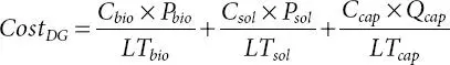
and the installation cost, considering the maximum sizes of DGs and shunt capacitors, is defined as
(1.22) 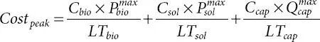
In this book chapter, equal preference is given to each objective function in the weighted sum approach. Therefore, the weights for the three objective functions are 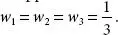
1.3.2 Technical Constraints Considered
The minimization of the weighted average of the three objective functions is subjected to the fulfilment of certain equality and inequality constraints as stated below [68],
(a) Equality Constraints
At any time instant t , the active and the reactive power balance for the distribution network should be maintained by the equation as follows
(1.23) 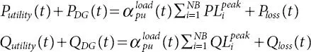
This equality constraint is fulfilled by the load flow solution of the distribution networks. Putility , Qutility are the active and reactive power taken from the utility, respectively, PDG, QDG are the active and reactive power supplied by the RDGs, in order, and shunt capacitors, and  is the percentage load level expressed in per unit.
(b) Inequality Constraints
(i) The bus voltages of the distribution networks at any time instant must be within the minimum (Vmin) and maximum (Vmax) voltage level as in(1.24)The placement of RDGs and the shunt capacitors may increase the bus voltage beyond the limit at low voltage level and decrease the bus voltage at high load level. Therefore, bus voltages are kept within the prescribed limit by introducing the penalty function defined as(1.25)
(ii) The active and reactive power generation of the DGs should be within the specified limit given as(1.26)where are the minimum and the maximum limit of the active power injection of the DGs and are the minimum and the maximum limit of the reactive power injection of the DGs which are to be maintained at any time instant. These inequalities are maintained by introducing the penalty function as below(1.27)
(iii) The total active and reactive power injections by the RDGs and shunt capacitors at any time instant should be less than the total active and reactive power load demand of the distribution network at the same instant. This inequality constraint is defined as(1.28)These inequality constraints are considered by introducing the two penalty functions as(1.29)
(iv) Branch currents, after the placement of DGs and shunt capacitors, should be within the maximum allowable level to maintain the feeder thermal limit. The branch current limit should be(1.30)This limit is considered in the objective function with the help of a penalty function described as(1.31)After considering all the penalty functions, the objective function, to be minimized, is(1.32)The values of the penalty factors τfeed are to be selected as very high value for a minimization problem. In this book chapter, the penalty values are selected as 1016 [68]. If any of the inequality constraints violates then the corresponding penalty function adds a very high value to the objective function.
1.4 Comparison of the SPBO Algorithm in Terms of CEC-2005 Benchmark Functions
For the comparison purpose, different algorithms ( viz . PSO [69], TLBO [70], CS, and SOS) are considered in this book chapter and the parameters for the different algorithms considered are tabulated in Table 1.2as below. The study has been carried out to analyze the performance of SPBO to solve CEC-2005 benchmark functions [67, 71]. The analysis has been done considering 30-dimensional problems. The comparison performance study of SPBO with PSO, TLBO, CS, SOS has been shown in Table 1.3. It may be noticed from Table 1.3, that the SPBO’s performance is better compared to that given by the remaining optimization algorithms considered. SPBO stands 1 strank in nine of benchmark functions of CEC-2005 according to the optimum solution achieved as well as based on converging mobility. The mean of the result obtained in nine benchmark functions is better as compared to the mean achieved by PSO, TLBO, CS and SOS. In only one function ( i.e . F8) SPBO stands 3 rd. Compared to the other algorithms considered in this analysis, it can be found in the study that the performance of the proposed SPBO algorithm is better.
Table 1.2 Parameters of different algorithms for benchmark functions.
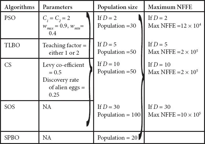
An entry “NA” means not applicable.
So, it may be inferred that the proposed novel SPBO method works fine to solve ten CEC-2005 benchmark functions considered in this book chapter.
1.5 Optimum Placement of RDG and Shunt Capacitor to the Distribution Network
In this current book chapter, optimum placement of RDG (biomass and solar PV) and shunt capacitor has been considered for the study purpose. The DG optimization problem may be divided into two sections, such as optimization of the location of DG and optimization of the size of DG. To optimize both the location and size of the DGs simultaneously, mixed discrete SPBO has been used in this study. In the mixed discrete SPBO, the sizes of the DGs are considered as the continuous variables, and locations of the DGs are considered as the discrete variables. To optimize the sizes and locations of the biomass, solar PV, and shunt capacitor, a multi- objective function is considered in this study. The objective function is described in (Equation 1. 12). The study has been carried out for a variable load demand for a day. Load demand of a network is not constant throughout the day. It varies with time, so as the power generation of the solar PV. Table 1.4shows the load demand and electrical power generation from the solar PV for a day. The graphical representation of the variation of load demand (pu) and power generation from PV (pu) with respect to the different load hours of a day has been portrayed in Figure 1.2.
Table 1.3 Optimization result of CEC-2005 benchmark functions.
| Functions | Attributes | PSO | TLBO | CS | SOS | SPBO |
|---|---|---|---|---|---|---|
| F1 | Best FF | -450.0000 | 4.3423×10 3 | 285.0288 | -450.0000 | -450.0000 |
| Worst FF | -450.0000 | 1.2868×10 4 | 2.6304×10 4 | -450.0000 | -450.0000 | |
| Mean | -450.0000 | 6.1561×10 3 | 9.2000×10 3 | -450.0000 | -450.0000 | |
| Std. Dev | 0 | 2.4294×10 3 | 8.1507×10 3 | 0 | 0 | |
| Rank | 3 | 5 | 4 | 2 | 1 | |
| F2 | Best FF | -450.0000 | -450.0000 | -450.0000 | -450.0000 | -450.0000 |
| Worst FF | -450.0000 | -450.0000 | -449.9989 | 7.8615×10 8 | -450.0000 | |
| Mean | -450.0000 | -450.0000 | -449.9998 | 7.8615×10 7 | -450.0000 | |
| Std. Dev | 0 | 0 | 3.3800×10 -4 | 2.3584×10 8 | 0 | |
| Rank | 2 | 3 | 4 | 5 | 1 | |
| F3 | Best FF | 2.4082×10 6 | 1.2404×10 7 | 2.7113×10 6 | 1.4156×10 6 | 1.1252×10 6 |
| Worst FF | 1.4310×10 7 | 9.0300×10 7 | 4.4354×10 6 | 6.8667×10 6 | 5.5039×10 6 | |
| Mean | 5.9320×10 6 | 7.4449×10 7 | 3.5213×10 6 | 3.0747×10 6 | 3.6913×10 6 | |
| Std. Dev | 3.6300×10 6 | 1.2404×10 7 | 7.8163×10 5 | 1.4156×10 6 | 1.2379×10 6 | |
| Rank | 3 | 5 | 4 | 2 | 1 | |
| F4 | Best FF | -450.0000 | -449.9981 | -450.0000 | -449.9957 | -450.0000 |
| Worst FF | -450.0000 | -449.7224 | -450.0000 | 1.025×10 9 | -450.0000 | |
| Mean | -450.0000 | -449.9655 | -450.0000 | 1.0264×10 8 | -450.0000 | |
| Std. Dev | 0 | 8.1216×10 -2 | 0 | 3.0745×10 8 | 0 | |
| Rank | 2 | 4 | 3 | 5 | 1 | |
| F5 | Best FF | 1.4051×10 4 | 1.0443×10 4 | 1.1914×10 4 | 7.9132×10 3 | 7.5236×10 3 |
| Worst FF | 3.6183×10 4 | 1.7420×10 4 | 5.3257×10 4 | 1.8809×10 4 | 9.7728×10 3 | |
| Mean | 2.3954×10 4 | 1.3856×10 4 | 2.8358×10 4 | 1.1950×10 4 | 8.4225×10 3 | |
| Std. Dev | 7.0703×10 4 | 2.2846×10 3 | 1.0637×10 4 | 3.2094×10 3 | 3.1287×10 3 | |
| Rank | 5 | 3 | 4 | 2 | 1 | |
| F6 | Best FF | 390.0070 | 405.8698 | 390.0033 | 390.0007 | 390.0002 |
| Worst FF | 462.3391 | 407.8258 | 449.3571 | 457.6640 | 390.0492 | |
| Mean | 412.4370 | 406.5812 | 403.1944 | 401.5661 | 390.0157 | |
| Std. Dev | 25.1252 | 0.5722 | 16.8726 | 18.9630 | 0.0176 | |
| Rank | 4 | 5 | 3 | 2 | 1 | |
| F7 | Best FF | -179.9926 | 4.2916×10 3 | -179.9926 | -179.9926 | -180.0000 |
| Worst FF | -179.9803 | 8.2175×10 3 | -179.9459 | -179.8050 | -179.9901 | |
| Mean | -179.9764 | 5.8506×10 3 | -179.9754 | -179.9596 | -179.9943 | |
| Std. Dev | 1.8121×10 -2 | 1.2183×10 3 | 1.7129×10 -2 | 5.3002×10 -2 | 3.7955×10⁻³ | |
| Rank | 2 | 5 | 3 | 4 | 1 | |
| F8 | Best FF | -119.5245 | -119.3254 | -119.9887 | -120.6199 | -119.5256 |
| Worst FF | -119.0590 | -119.0550 | -119.9010 | -120.2961 | -119.3143 | |
| Mean | -119.2094 | -119.1229 | -119.9549 | -120.4613 | -119.3801 | |
| Std. Dev | 0.1392 | 7.3253×10 -2 | 2.3401×10 -2 | 0.1028 | 7.3663×10 -2 | |
| Rank | 4 | 5 | 2 | 1 | 3 | |
| F9 | Best FF | -321.0454 | -164.8339 | -172.7972 | -293.1865 | -330.0000 |
| Worst FF | -302.1412 | -129.4599 | -55.3934 | -184.5407 | -330.0000 | |
| Mean | -313.3842 | -147.5225 | -123.7465 | -241.1199 | -330.0000 | |
| Std. Dev | 5.4141 | 11.0234 | 41.4742 | 42.6722 | 0 | |
| Rank | 2 | 4 | 5 | 3 | 1 | |
| F10 | Best FF | -217.5703 | -150.7517 | -100.1658 | -225.9089 | -256.3699 |
| Worst FF | -92.2075 | -104.3583 | 91.8576 | -100.6526 | -184.7313 | |
| Mean | -153.3029 | -125.7336 | -9.2147 | -151.2863 | -213.3927 | |
| Std. Dev | 38.9758 | 14.0585 | 62.1465 | 38.1157 | 17.6163 | |
| Rank | 3 | 4 | 5 | 2 | 1 |
For the study purpose, two different distribution networks are considered. The first distribution network is a 33-bus distribution network having a total active power demand of 3715 kW with active power loss of 202.6771 kW [65] at the peak load level. The other one is 69-bus distribution network having active power demand as 3802.2 kW and, reactive power demand as 2694.6 kVAr [67]. The active power loss at the peak load level of the 69-bus distribution network is 224.96 kW.
Читать дальшеИнтервал:
Закладка:
Похожие книги на «Intelligent Renewable Energy Systems»
Представляем Вашему вниманию похожие книги на «Intelligent Renewable Energy Systems» списком для выбора. Мы отобрали схожую по названию и смыслу литературу в надежде предоставить читателям больше вариантов отыскать новые, интересные, ещё непрочитанные произведения.


Обсуждение, отзывы о книге «Intelligent Renewable Energy Systems» и просто собственные мнения читателей. Оставьте ваши комментарии, напишите, что Вы думаете о произведении, его смысле или главных героях. Укажите что конкретно понравилось, а что нет, и почему Вы так считаете.