Daniel D. Stancil - Principles of Superconducting Quantum Computers

(1.51)

The matrix representation of the CNOT gate in this alternate convention is

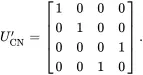(1.52)

We will consistently use the first convention, with the least-significant qubit (top-most on a circuit diagram) on the right when writing state labels.

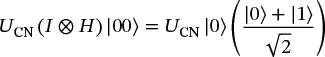
Consider the circuit shown in Figure 1.5. The circuit can be described mathematically as U CN( I ⊗ H ) |00⟩. Here the expression I⊗H simply means a Hadamard gate is applied to the right qubit, and the identity matrix applied to the left qubit (which leaves the left qubit unchanged). Completing the calculation gives

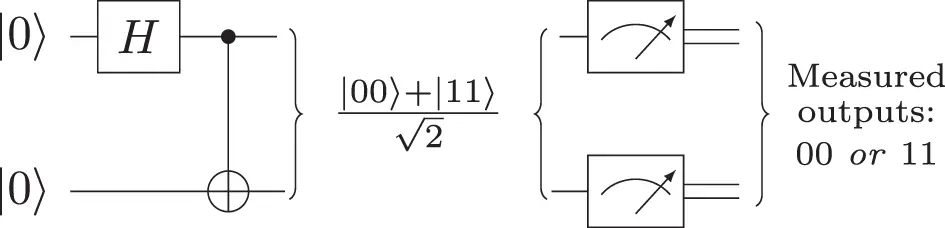
Figure 1.5 Circuit for creating an entangled state known as a Bell State. When the two qubits are measured, they will either both be 0, or they will both be 1.

(1.53)

(1.54)

(1.55)

Note that there is no way to factor this state into (qubit 1 state) ⊗ (qubit 0 state). This is known as a Bell State , and it is an example of an entangled state, as described in Section 1.1.5.

If we measure the state of one of the qubits in ( 1.55), then we will obtain either a zero or a one with equal probability, as we would expect. The unusual behavior happens when we measure the second qubit: if we measure |0⟩ on the first qubit, then we know the state has collapsed to |00⟩, so a measurement of the second qubit will also yield |0⟩. Similarly, if the first measurement yields |1⟩, then the state must have collapsed to |11⟩, so a measurement of the second qubit will also yield |1⟩. The measurements are correlated, no matter how far apart the physical qubits might be.

We simulated the Bell circuit using IBM’s Qiskit [2], and also executed the circuit on real IBM Quantum hardware. A histogram illustrating the results of simulating the circuit 1024 times (each execution is referred to as a “shot”) is shown in Figure 1.6. From ( 1.55), we see that the probability amplitudes of the states |00⟩ and |11⟩ are both equal to 1/2. Since the probability of measuring a state is the absolute magnitude squared of the amplitude, the probability of measuring each state is 1/2. Consistent with this, the measurements from the 1024 shots are roughly equally divided between the states |00⟩ and |11⟩, with no other states occurring.

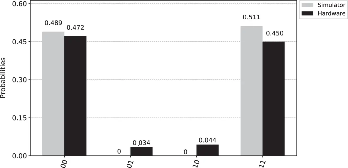
Figure 1.6 Result of executing the circuit 1024 times on a quantum simulator, compared with executing the circuit 1024 times on a real IBM quantum computer.

The simulator gives the result expected from an error-free quantum processor. In contrast, the quantum processors available today are noisy and contain errors. As an illustration, Figure 1.6 also shows the result of executing 1024 shots on a real IBM Quantum processor. Although the states |00⟩ and |11⟩ do occur most frequently, the error states |01⟩ and |10⟩ occasionally occur as well. Fortunately there are techniques to reduce and partially mitigate such noise ( Chapter 9), and these techniques represent an active area of research.

With a better understanding of quantum states and operations, we are now ready to construct a proof of the no-cloning theorem. The proof relies on the fact that unitary operators are linear ; when applied to a sum of states, the operator operates independently on each component:

(1.56)

Suppose we have an operator U clonethat takes two qubits, as shown in Figure 1.7. When the second qubit is |0⟩, it is replaced with an exact copy of the first qubit. The proof will show that such an operator cannot exist, because it is not compatible with the principle of linearity.

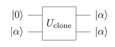
Figure 1.7 Hypothetical cloning operator, that creates an exact and independent copy of unknown quantum state | α ⟩. The text will show that such an operator cannot be implemented.

Further suppose that we have two states:

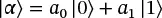(1.57)

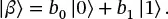(1.58)

By the definition of cloning:

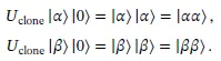(1.59)

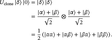
Now consider a new state |δ⟩=(|α⟩+|β⟩)/2. By the definition of cloning:

(1.60)

However, by the linearity of unitary operators:

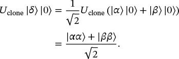(1.61)

Since Eqs. ( 1.60) and ( 1.61) cannot both be true, there is no unitary U clonethat can perform the cloning operation for all states.

We stated earlier that we can clone a (computational) basis state. This can be done with the CNOT gate, with the first qubit as the control. (With our bottom-to-top ordering, this corresponds to the UCN′ operator from ( 1.52).) Suppose state | ψ ⟩ is either |0⟩ or |1⟩, but we don’t know which.

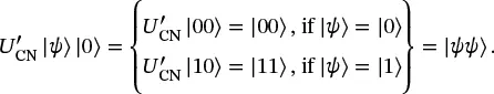(1.62)

If we apply the circuit from Figure 1.5 to an arbitrary state | ψ ⟩ = α |0⟩ + β |1⟩, we get a result that looks sort of like cloning, but not quite:

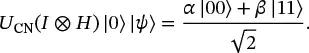(1.63)