Daniel D. Stancil - Principles of Superconducting Quantum Computers

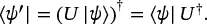
Since the length of the state vector must always be unity, we are only allowed to use matrices U that conserve the length of the vector. In other words, ⟨ ψ ′| ψ ′⟩ = ⟨ ψ | ψ ⟩ = 1. This puts a very important constraint on the matrix U :

(1.15)

using the following observation:

(1.16)

Since ⟨ ψ | ψ ⟩ = 1, we conclude that

(1.17)

where I is the identity matrix

(1.18)

Matrices that satisfy this requirement are called unitary matrices. We can view these matrices as performing an operation on a qubit by changing the mixture of basis states. Consequently, the matrices U are also referred to as unitary operators .

The identity matrix I can be considered to be the simplest “gate” and leaves the state vector unchanged. Classically, the NOT gate is the only non-trivial single-bit gate. In contrast, there are many non-trivial single qubit quantum gates (technically, the number of 2×2 unitary matrices is unlimited). The most common non-trivial single qubit gates are the Pauli-X ( X ), Pauli-Y ( Y ), Pauli-Z ( Z ), and Hadamard ( H ) gates defined as follows:

(1.19)

(1.20)

(1.21)

(1.22)

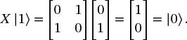
To get an understanding of what these gates do, consider applying an X gate to the “ground” state |0⟩:

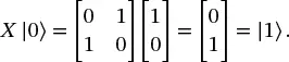(1.23)

Similarly,

(1.24)

We see then that the X gate is a “bit flip” gate, and transforms |0⟩ into |1⟩ and vice versa. This, then is the analog of the classical NOT gate. You should verify the following results from applying Y,Z, and H gates:

(1.25)

(1.26)

(1.27)

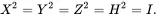
In addition, it is interesting to note that each one of these matrices is its own Hermitian conjugate. Consequently, these four gates have the property that applying them twice gives the identity matrix:

(1.28)

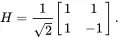
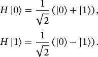
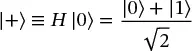
Note that while X,Y, and Z gates transform between the |0⟩ and |1⟩ states, the Hadamard gate actually creates a superposition state, and therefore will prove to be particularly useful. The states resulting from applying H to the basis states are given their own names:

(1.29)

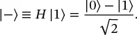(1.30)

Multiple gates can be sequentially applied to a qubit by matrix multiplication:

(1.31)

This expression says that we start with the ground state, then apply a Hadamard gate, followed by a Pauli-Y and then a Pauli-Z. Note that this process conceptually moves from right to left. This computation can be represented by a quantum circuit diagram as shown in Figure 1.3. Note that the process moves from left to right on the circuit diagram: we begin with the ground state on the left, then apply a Hadamard gate, a Pauli-Y gate, and a Pauli-X.

Figure 1.3 Circuit representation of Eq. ( 1.31). In a quantum circuit diagram, the operation goes from left to right, while the matrix expression is shown going from right to left. The final box is a measurement in the standard basis, resulting in a classical bit.

Finally, after performing a quantum calculation, we generally measure each qubit. The symbol for a measurement is shown as the last element in Figure 1.3. This action collapses the final state onto one of the basis states. The outcome of a measurement is a classical bit that is stored in a classical register. “Quantum wires” are denoted by solid lines, and “classical wires” are denoted with double lines. A quantum wire simply represents a time-interval over which the state is kept unchanged.

It is also possible to have gates with multiple qubits as inputs. However, unlike classical multi-bit gates, the fact that quantum gates are reversible requires that there must be the same number of output qubits as input qubits. In this section we will explore some common two-qubit gates.

When we consider a system with two qubits, we don’t just consider each qubit independently of the other. Instead, this forms a two-qubit system with its own set of basis states. If we know the state of each qubit, then the combined two-qubit state is described using the tensor product of the two state vectors, defined as follows:

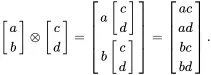(1.32)