Neil McCartney - Properties for Design of Composite Structures

(4.31)

(4.32)

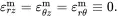
It follows directly from ( 4.17), ( 4.30) and ( 4.32) that for fibre and matrix

(4.33)

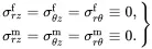
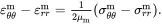
On subtracting ( 4.14) and ( 4.15), it follows that for fibre and matrix

(4.34)

(4.35)

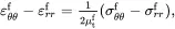
Relations ( 4.29) and ( 4.31) then assert that

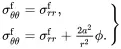(4.36)

On substituting ( 4.33) and ( 4.34) into the equilibrium equations ( 4.20)–( 4.22) it follows that

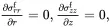(4.37)

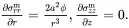(4.38)

On integrating ( 4.38) 1subject to the condition ( 4.28) 1,

(4.39)

and from ( 4.36) it follows that

(4.40)

On integrating ( 4.37) 1using ( 4.39) together with the continuity condition ( 4.28) 3

(4.41)

and from ( 4.36) it follows that

(4.42)

The substitution of ( 4.29) 3, ( 4.41) and ( 4.42) into ( 4.16) leads to

(4.43)

It is clear from ( 4.41) that σzzf is a constant, automatically satisfying ( 4.37) 2. The substitution of ( 4.31) 3, ( 4.39) and ( 4.40) into ( 4.16), applied to the matrix, leads to

(4.44)

thus automatically satisfying ( 4.38) 2. The substitution of ( 4.29), ( 4.31), ( 4.39)–( 4.44) into relation ( 4.14), applied to the fibre and matrix, leads to

(4.45)

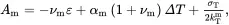(4.46)

where kTf is the plane strain bulk modulus for the transverse isotropic fibre and kTm is the plane strain bulk modulus of the isotropic matrix, defined by (see (2.202))

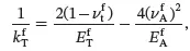(4.47)

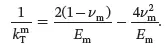(4.48)

It should be noted that

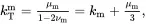(4.49)

where km is the bulk modulus of the matrix defined by (see (2.205))

(4.50)

It now only remains to determine the constant ϕ , which can be specified on applying the remaining condition ( 4.28) 5, because the conditions ( 4.28) 2, ( 4.28) 4and ( 4.28) 6are automatically satisfied by ( 4.25) and ( 4.33). It follows from ( 4.26), ( 4.27), ( 4.28) 5, ( 4.45) and ( 4.46) that

(4.51)

where

(4.52)

The displacement distribution is specified by ( 4.25)–( 4.27), and the corresponding stress distribution is specified by ( 4.33), ( 4.39)–( 4.44). The stress-strain relations ( 4.14)–( 4.17) and the equilibrium equations ( 4.20)–( 4.22) are satisfied exactly. The boundary and interface conditions ( 4.28) are also satisfied exactly.

For the general loading conditions characterised by the parameters ε, σT and ΔT and applied to an infinite sample of matrix in the absence of fibre (filling the entire region of space) the solution is given by

(4.53)

(4.54)

where the parameter Am is given by ( 4.46). It should be noted that the axial stress in the matrix given by ( 4.54) 2is identical to that in the matrix when the fibre is present (see ( 4.44)). It should also be noted that when the fibre is introduced the radial displacement function is perturbed as a second term appears in ( 4.27) 1that is inversely proportional to the radial distance r . This additional term will now be considered when applying Maxwell’s method of estimating the properties of a fibre-reinforced composite.

Owing to the use of the far-field in Maxwell’s method for estimating the properties of fibre composites, it is possible to consider multiple fibre reinforcements. Suppose in a cluster of fibres that there are N different types such that for i = 1, …, N there are ni fibres of radius ai. The properties of the fibres of type i are denoted by a superscript i . The cluster is assumed to be homogeneous regarding the distribution of fibres, and leads to transverse isotropic effective properties.