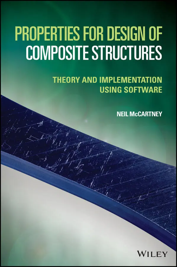
Neil McCartney - Properties for Design of Composite Structures

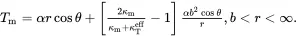
(4.8)

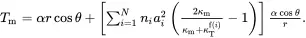
The cluster of all types of fibre is now considered to be enclosed in a cylinder of radius b such that the volume fraction Vfi of fibres of type i within the cylinder of radius b is given by ( 4.1). On using ( 4.7) the temperature distribution in the matrix outside the cylinder of radius b is then given by

(4.9)

The second stage is to equate the perturbation terms in ( 4.8) and ( 4.9) (i.e. the second terms on the right-hand side) so that, on using ( 4.1), the effective thermal conductivity of the multiphase cluster of fibres may be obtained from the relation

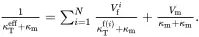(4.10)

The effective thermal conductivity of the multiphase fibre composite is then given by

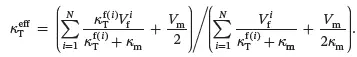(4.11)

The bounds for the conductivity of a multiphase composite are given by Torquato [5] which may be written in the following simpler form, having the same structure as the result ( 4.10) derived using Maxwell’s methodology

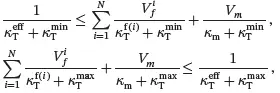(4.12)

where κmin is the lowest value of conductivities for all phases, whereas κmax is the highest value.

The effective axial thermal conductivity of the unidirectional composite is given by the following mixtures rule

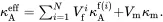(4.13)

The validity of this relationship arises from the fact that the temperature distribution is such that there is no heat flow across the fibre/matrix interfaces. The temperature is linear in the axial direction having the same gradient in both fibre and matrix.

When considering an isolated cylindrical fibre embedded in matrix material, it is convenient to introduce a set of cylindrical polar coordinates (r,θ,z) where the origin lies on the axis of the fibre. All fibres are assumed to be made of transverse isotropic solids where properties are isotropic in the plane normal to the fibre axes. When using cylindrical polar coordinates, transverse isotropic solids (see (2.199)) are characterised by stress-strain relations of the form

(4.14)

(4.15)

(4.16)

(4.17)

(4.18)

Superscript ‘f’ is used to denote anisotropic fibre properties and subscript ‘m’ is used to denote the properties Em, νm, μm and αm of an isotropic matrix such that Em=2μm(1+νm). If the fibres are also isotropic then

(4.19)

The equilibrium equations for the fibres and matrix in the absence of body forces are (see (2.125)–(2.127))

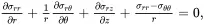(4.20)

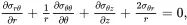(4.21)

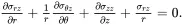(4.22)

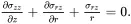
The following analysis applies to an isolated cylindrical fibre of radius a that is perfectly bonded to an infinite matrix, subject to a uniform temperature change Δ T , where the system is subject to a uniform axial strain ε and a uniform transverse stress σT. The equilibrium equations ( 4.20)–( 4.22) for the fibre and matrix, assuming symmetry about the fibre axis so that stress components are independent of θ and the shear stresses σrθ and σθz are zero, then reduce to the form

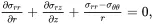(4.23)

(4.24)

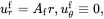
In regions away from the loading mechanism it is reasonable to assume that

(4.25)

where ε is the axial strain applied to the composite. A solution is now sought of the following classical Lamé form

(4.26)

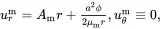(4.27)

where A f, A mand ϕ are constants to be determined.

The boundary and interface conditions that must be satisfied are

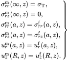(4.28)

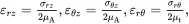
On differentiating the displacement field, it follows, on using (2.139) on setting uθ≡0, that.

(4.29)

(4.30)