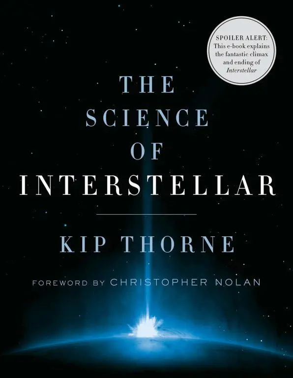
Kip Thorne - The Science of Interstellar

The equations that I gave to Oliver James at Double Negative, for the orbital motion of light rays around Gargantua, are a variant of those in Appendix A of Levin and Perez-Giz (2008). Our equations for the evolution of bundles of rays are a variant of those in Pineult and Roeder (1977a) and Pineult and Roder (1977b). In several papers that we’ll make available at http://arxiv.org/find/gr-qc, Paul Franklin’s team and I give the specific forms of our equations and discuss details of their implementation and the simulations that resulted.

Here are the calculations that underlie my statements in Chapter 13. They are a nice example of how a scientist makes estimates. These numbers are very approximate; I quote them accurate to only one digit.

The mass of the Earth’s atmosphere is 5 × 10 18kilograms, of which about 80 percent is nitrogen and 20 percent is molecular oxygen, O 2—that is, 1 × 10 18kilograms of O 2. The amount of carbon in undecayed plant life (called “organic carbon” by geophysicists) is about 3 × 10 15kilograms, with roughly half in the oceans’ surface layers and half on land (Table 1 of Hedges and Keil [1995]). Both forms get oxidized (converted to CO 2) in about thirty years on average. Since CO 2has two oxygen atoms (that come from the atmosphere) and just one carbon atom, and the mass of each oxygen atom is 16/12 that of a carbon atom, the oxidization of all this carbon, after all plants die, would eat up 2 × 16/12 × (3 × 10 15kilograms) = 1 × 10 16kilograms of O 2, which is 1 percent of the atmosphere’s oxygen.

For evidence of sudden overturns of the Earth’s oceans and the theory of how they might be produced, see Adkins, Ingersoll, and Pasquero (2005). The standard estimate of the amount of organic carbon in sediments on the ocean bottoms that might be brought to the surface by such an overturn focuses on an upper sedimentary layer that is mixed by ocean currents and animal activity. This mixed layer’s carbon content is the product of an estimated rate of deposit of carbon into the sediments (about 10 11kilograms per year) and the average time it takes for its carbon to be oxidized by oxygen from ocean water (1000 years), giving 1.5 × 10 14kilograms, one-twentieth of that on land and in ocean surface layers (Emerson and Hedges 1988, Hedges and Keil 1995). However: (i) The estimated deposition rate could be wrong by a huge amount; for example, Baumgart et al. (2009), relying on extensive measurements, estimate a deposition rate in the Indian Ocean off Java and Sumatra that is uncertain by a factor of fifty and, extrapolated to the whole ocean could give as much as 3 × 10 15kilograms of carbon in the mixed layer (the same as on land and in the ocean’s surface layers). (ii) A substantial fraction of the deposited carbon could sink into a lower layer of sediment that does not get mixed into contact with seawater and oxidized except possibly during sudden ocean overturns. The last overturn is thought to have been during the most recent ice age, about 20,000 years ago—twenty times longer than the oxidation time in the mixed layer. So the unmixed layer could have twenty times more organic carbon than the mixed layer, and as much as twenty times that on land and in the ocean’s surface. If brought to the ocean surface by a new overturn and there oxidized, this is nearly enough to leave everyone gasping for oxygen and dying of CO 2poisoning; see the end of Chapter 12. Thus such a scenario is conceivable, though highly unlikely.

Christopher Nolan chose several kilometers for the diameter of Interstellar ’s wormhole. The wormhole’s angular diameter as seen from Earth, in radians, is this diameter divided by its distance from Earth, which is about 9 astronomical units or 1.4 × 10 9kilometers (the radius of Saturn’s orbit). Therefore, the wormhole’s angular diameter is about (2 kilometers)/(1.4 × 10 9kilometers) = 1.4 × 10 –9radians, which is 0.0003 arc-seconds. Radio telescopes routinely achieve this angular resolution using transworld interferometry. Optical telescopes on the ground using a technique called “adaptive optics,” and the Hubble space telescope in space, achieve angular resolutions a hundred times worse than this in 2014. Interferometry between twin Keck telescopes in Hawaii in 2014 can achieve a resolution ten times worse than the wormhole’s angular diameter, and it is very plausible that in the era of Interstellar optical interferometry between more widely spaced optical telescopes will make possible resolutions better than the wormhole’s 0.0003 arc-seconds.

If you are familiar with Newton’s gravitational laws in mathematical form, then you may find it interesting to explore a modification of them by the astrophysicists Bohdan Paczynski and Paul Wiita (Paczynski and Wiita 1980). In this modification, the gravitational acceleration of a nonspinning black hole is changed from Newton’s inverse square law, g = GM / r 2to g = GM /( r – r h ) 2. Here M is the hole’s mass, r is the radius outside the hole at which the acceleration g is felt, and r h = 2 GM / c 2is the radius of the nonspinning hole’s horizon. This modification is a surprisingly good approximation to the gravitational acceleration predicted by general relativity. [60] This Paczynski-Wiita modification of gravity was used in developing the black hole’s influence on spacecraft orbits for a gravitational-slingshot video game associated with Interstellar ; see Game.InterstellarMovie.com . Using this modified gravity, can you give a quantitative version of Figure 17.2 [61] For a related calculation, see the technical notes for Chapter 27, below. and deduce the radius of the orbit of Miller’s planet? Your result will be only roughly correct, because the Paczynski-Wiita description of Gargantua’s gravity fails to take account of the dragging of space into a whirling motion by the black hole’s spin.

The meaning of the various mathematical symbols that appear in the Professor’s equation (Figure 25.6) is explained on his other fifteen blackboards, which can be found on the web at this book’s page at Interstellar.withgoogle.com. His equation expresses an “Action” S (the classical limit of a “quantum effective action”) as an integral over “Lagrangian” functions L. These Lagrangians involve the spacetime geometries (“metrics”) of the five-dimensional bulk and our four-dimensional brane, and also involve a set of fields that live in the bulk (denoted Q , σ, λ, ξ, and φ i ), and also “standard model fields” that live in our brane (including the electric and magnetic fields). The fields and spacetime metrics are to be varied, seeking an extremum (maximum or minimum or saddle point) of the Action S . The conditions that produce an extremum are a set of “Euler-Lagrange” equations that control the evolutions of the fields. This is a standard procedure in the calculus of variations. The Professor and Murph make guesses for a list of unknown bulk fields φ i and unknown functions U ( Q ), H ij ( Q 2), M (standard model fields), and unknown constants W ij that appear in the Lagrangian. In Figure 25.9 you see me writing a list of their guesses on the blackboard. Then for each set of guesses, they vary the fields and spacetime geometries, deduce the Euler-Lagrange equations, and then explore in computer simulations those equations’ predictions for the gravitational anomalies.