John Crisp - Introduction to Microprocessors and Microcontrollers

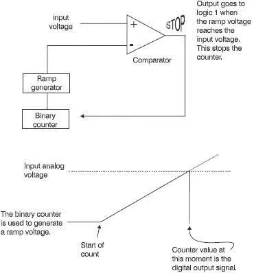
Figure 17.3 An ADC that uses a ramp voltage

Successive approximation

If we were to use a 3-bit digital signal to convert an analog voltage of between 0 V and 4 V we could have the 3 bits representing voltages of 4 V, 2 V and 1 V. This is how the circuit responds to an input of 3.5 V.

The digits are initially set to 000. The left-hand bit is switched on and its 4 V is compared with the input. The input is seen to be less than this so this digit is reset to zero. It then tries the next bit and its 2 V are compared and found to be less than the input so it remains set. The digital signal is now 010. The circuit now adds the 1 V from the last digit. The result is a total of 3 V, which is compared with the input analog signal. The input of 3.5 V still exceeds the current value of 3 V so the last bit is set. The final digital output is 011.

The circuit has tried all the available values until it finds the one that provides the result closest, but less than the input signal. As before, the more bits we are using, the more accurate is the result.

In checking the specifications of likely ADCs to use, we need to compare the following criteria.

Quantization error

In the above example using the flash converter, we can see that an analog input of 3.5 V would provide the same output as would any value between slightly over 3 V and slightly less than 4 V. This error means that small variation in the analog input voltage will be lost. The size of this error is equal to the space between the comparator reference voltages.

Changing from eight comparators to 1024, would mean that the voltage gaps would decrease from 1 V to 7.8 mV as would the quantization error. Regardless of the method used for A–D conversion, quantization error is always present.

Bits

The more bits, the merrier. Likely values will be between 8 and 16.

Speed

There are two factors here. How often can we get an updated value for the signal and how well can we follow any changes it is making? Even if we do not want the signal to be sampled at a very high rate, we still may want to take a quick sample so that the input value is unlikely to change very much as the sample is actually being measured.

For speed, you cannot beat the flash converter. It can sample for a period as short as 3 ns which compares very favourably with the typical values of 10 μs for the ramp generators and successive approximation types.

Changing a group of digital bit values to an analog voltage is basically just the reverse process of the A–D conversion that we met in the previous section.

Most digital to analog converters operate by adding current together then converting the result into an analog voltage. The binary levels are used to switch currents on or off.

Let’s assume a 4-bit digital signal in which the most significant bit is made to generate a current of 8 mA and the others produce, in turn, 4, 2 and finally 1 mA. If the digital signal to be converted happened to be 10112, then the first, third and fourth current sources would be activated giving a total of 8+2+1=11 mA (Figure 17.4).

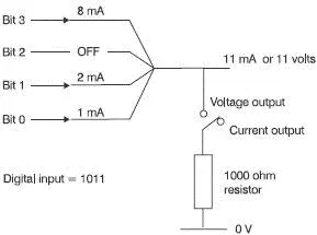
Figure 17.4 A DAC with a current or voltage output

In some DACs the final output is a changing current but in others it has been converted to a variable voltage. It just depends on which integrated circuit you choose to use. In the ones offering a voltage output, the total current is then passed through a resistor. If we choose a nice easy value like 1 kΩ, the voltage across the resistor would be 11 mA×1 kΩ=11 V.

In a similar way, we can see that all binary values between 0000 and 1111 would be converted into voltages between 0 V and 15 V. There are a couple of specifications that may need to be checked to decide on which one to use.

Resolution

This is the number of digital bits used to convert into an analog voltage. Typical values available are from 4 to 18 bits. As the digital input changes by a single bit, say from 1000 to 1001, the resultant voltage or current increases by a discrete step. The size of this step is determined by the number of bits used compared with the maximum value of the output current or voltage.

For example, if we used 4 bits then this would provide a total of 16 different steps and if the maximum happened to be 8 V, each step will represent a voltage change of 0.5 V. Thus, a steadily increasing digital signal will cause the analog voltage to increase in small discrete steps like a staircase. This is all very similar to the cause of quantization error.

Speed

The speed of operation is very dependent on the chip being considered. The conversion times available from an exceedingly fast 1 ns to a sluggish 5 μs.

In sending information in digital form, we have a choice of using serial or parallel transmission. In the case of serial transmission, the binary values are represented by two different voltage levels and are sent one after the other along a cable. This is simple but slow. The alternative is to have several wires and thus be able to send several bits of data at the same time, one on each conductor.

In a microprocessor-based system, even if it is a one-off, it is usually better to conform to established standards for the cabling so that other instruments and circuits can be connected with a minimum of hassle.

Parallel connection

There are several different standards used for parallel connection of data but one of the most widely used, and most reliable, was produced by Centronics.

The Centronics system sends eight bits at a time and employs a 36 plug and socket system. To send data, there are four basic control signals as well as the eight data lines. It also stipulates a variety of other control wires that can be used if required.

The important thing to remember about these standards is that you do not have to use all the connections listed but those that you do decide to use should conform to the stated specification and be on the correct pins. This ensures that if the plug is inserted into a new piece of equipment, it may not work but at least it will not be damaged.

Centronics data transmission

To see how the system works, we will use timing diagrams to show what happens and when. These diagrams, which all look very similar at first glance, are shown in all data manuals to show the sequence of events inside the microprocessor and in the surrounding circuit.

There are a couple of points that are worth mentioning. We have mentioned the problem of rise time in Chapter 7. You will remember that we cannot change a voltage level instantaneously. It may not seem an important delay when we think of switching a light on at home but when the microprocessor is handling data at millions of bits per second, these delays can be important and is a common cause of failure in a circuit that ‘should’ work. Most waveform diagrams show the ends of a square wave as sloping lines rather than vertical ones.

In Figure 17.5 we have a positive-going pulse to represent a data value of 1 but, of course, data could equally well be at 0 V to represent a binary 0. In cases where we want to show that a level has changed, but it may go to either level, we redraw the diagram to show both possibilities at the same time, as in Figure 17.6.

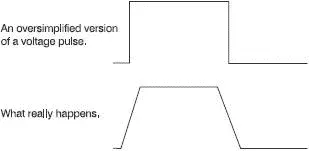
Figure 17.5 Rise and fall time may be important