John Crisp - Introduction to Microprocessors and Microcontrollers

1 0 1 1

The top row now has an even number of ‘1’s. The next row has four ‘1’s which is an even number so we do not need to add another ‘1’. We therefore add a ‘0’:

0 0 1 0 1

1 1 1 1 0

0 1 0 1

1 0 1 1

The third row will be completed with a ‘0’ since it contains an even number of ‘1’s and the last row, with three ‘1’s will need an extra one to be added. The result is now:

0 0 1 0 1

1 1 1 1 0

0 1 0 1 0

1 0 1 1 1

Step 3 We now have five columns down the page and we can add extra ‘1’s in the same way to make the total number of ‘1’s an even number. The first two and the last columns each contain two ‘1’s so zeros will be added. The third and fourth columns have three ‘1’s so we need to add an extra ‘1’ to each. The result is now:

0 0 1 0 1

1 1 1 1 0

0 1 0 1 0

1 0 1 1 1

0 0 1 1 0

Notice how we have now got a total of 25 bits to be transmitted. This represents 16 bits of data and 9 bits added to check the accuracy of the data. The final serial transmission is 0010111110010101011100110. This means that 9 out of 25 or 36% of the transmission is not actual data and represents redundancy.

Let’s see how it works. We will assume an error has occurred and one of the bits is received incorrectly so here is the received transmission:

0010111110010101001100110

Step 1 Layout the data as a 5×5 square.

0 0 1 0 1

1 1 1 1 0

0 1 0 1 0

1 0 0 1 1

0 0 1 1 0

Step 2 Check the parity in each row across the square. We decided to make each row and column to have an even parity.

The first row has two ‘1’s, this is even – OK.

The second row has four ‘1’s, this is even – OK.

The third row has two ‘1’s, this is even – OK.

The fourth row has three ‘1’s, this is odd – an error has occurred.

The last row has two ‘1’s, this is even – OK.

We now know that one of the bits in the fourth row has been received incorrectly.

Step 3 Do the same for the columns.

The first column has two ‘1’s, this is even – OK.

The second column has two ‘1’s, this is even – OK.

The third column has three ‘1’s, this is odd – an error exists in column three.

The fourth column has four ‘1’s, this is even – OK.

The last column has two ‘1’s, this is even – OK.

Step 4 Isolate the error and change the data.

The error occurs in the third column and the fourth row. Since this is now known to be an error and we only have a choice of 0 or 1, we can confidently change the 0 to a 1 and recover the correct data stream.

0 0 1 0 1

1 1 1 1 0

0 1 0 1 0

1 0 11 1

0 0 1 1 0

In this example, we chose to use even parity, that is, we made each row and column have an even number of ‘1’s. It would work equally well if we used odd parity by making the number of ‘1’s an odd number. It would also work just as well if we counted the zeros instead of the ones. If more than one error occurs, it will warn us of an error but it will be unable to make any corrections. If you try it, you will see that it indicates four possible positions for the two errors and nine for three errors.

Example

Correct this received data which includes one error. To provide automatic correction, odd parity on the ‘1’s has been used.

The received signal: 1101001001111001010101101.

Step 1 Layout the data as a 5×5 square

1 1 0 1 0

0 1 0 0 1

1 1 1 0 0

1 0 1 0 1

0 1 1 0 1

Step 2 Check the columns and rows for an odd number of ‘1’s

1 1 0 1 0 ✓

0 1 0 0 1 ×

1 1 1 0 0 ✓

1 0 1 0 1 ✓

0 1 1 0 1 ✓

✓ × ✓ ✓ ✓

Step 3 Isolate the error

1 1 0 1 0 ✓

0 10 0 1 ×

1 1 1 0 0 ✓

1 0 1 0 1 ✓

0 1 1 0 1 ✓

✓ × ✓ ✓ ✓

Step 4 The data where the column and row intersect is the error. So we simply change the ‘1’ to a ‘0’.

Step 5 Strip out the parity bits to recover the original data

11010000111010100110

The most basic way of sending information from one place to another is simply to connect a wire to both ends of the system and apply a voltage to one end. By making the voltage vary, we can send different levels and even speech or music. These are called analogue signals and have many drawbacks.

The main one is the effect of noise. As the signal travels along a wire it gets weaker and it has noise induced into it by random electromagnetic signals and vibration of the molecules of the conductor. The overall effect is that the signal becomes degraded and weaker.

The ‘weaker’ bit is no problem, we can soon amplify it back to its original size but the noise is a different matter. The electrical noise has become embedded into the signal and has permanently distorted it. Amplifying it will amplify the noise and the signal equally.

We have no problem with digital signals since we know that they will all be rectangular in shape and so the amplifier can be used to regenerate the shape of the signal and hence strip out the effects of the noise. If we are faced with sending something inherently analogue, like speech or music, our first job is to convert it to a digital form.

Inevitably these days, this is taken care of by an integrated circuit of which there are many different designs. It is quite possible, but totally uneconomic, to construct our own ADC so it is really a matter of flicking through the catalogues and choose the most appropriate one available.

There are several different designs of ADCs, which are based on three basically different approaches.

Flash converter

The first is called a flash converter or parallel encoder. These use circuits called comparators. A comparator has two inputs, one is the analogue voltage being converted and the other is a known reference voltage.

All we ask of a comparator is to answer a simple question: ‘Is the analogue input voltage higher or lower than our reference voltage?’ It answers by changing its output voltage to a logic 1 to mean it is higher and a logic 0 to mean it is lower. They are so accurate that the chance of it accepting the two voltages as the same level are extremely slight and doesn’t happen in practice (see Figure 17.2).

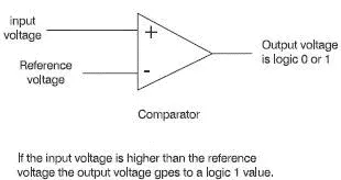
Figure 17.2 A comparator used in a flash ADC

So how do we use the comparator? If we had three of them with reference voltages set to 1 V, 2 V and 3 V and then applied the input voltage of 2.5 V to all of them, the first two would set their outputs to a level 1 and the last one would be unaffected at logic 0. The logic levels could be used to generate a binary number to represent 2.5 V.

An input voltage of 2.4 V or 2.9 V would also result in the same comparators being activated and hence the same output digital signal. This error occurs in all analog to digital converters. We can reduce the size of the error by increasing the number of comparators to detail more levels. Real ones have between 16 and 1024 different levels.

Ramp generators

These are a combination of a binary counter that simply counts up from zero to its maximum value, perhaps 1024 like the last type. As the binary count proceeds, a ramp voltage is made to steadily increase. A single comparator is used to compare the output of the ramp voltage with the analog voltage being converted. As soon as the ramp voltage exceeds the input voltage, the comparator signal stops the counter. The counter output is then the digital equivalent of the analog signal (see Figure 17.3).