Robert G. Reynolds - Cultural Algorithms

The shape of the network varies based on the selection made by the user, varying how each agent is able to communicate with its neighbors, and how far information can penetrate the social network. As we can see in Figure 2.11, in a homogeneous topology, all neighbors have an equivalent level of connectedness to all other neighbors. If any given agent has four connections in a homogeneous network topology, then ALL agents have four connections in a homogeneous network topology. Heterogeneity in network topologies can be seen in the uses of subcultures, in which network connections are awarded based on agent merit, and in randomization, in which each agent has access to a random number of others as discussed next in Chapter 3.

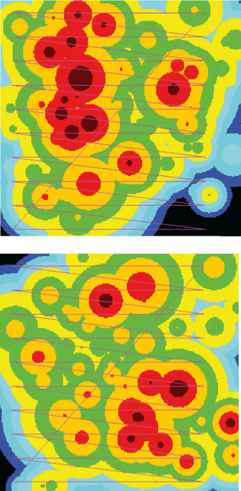
Figure 2.9 The initialization stage of the static (above) and dynamic (below) landscape runs.

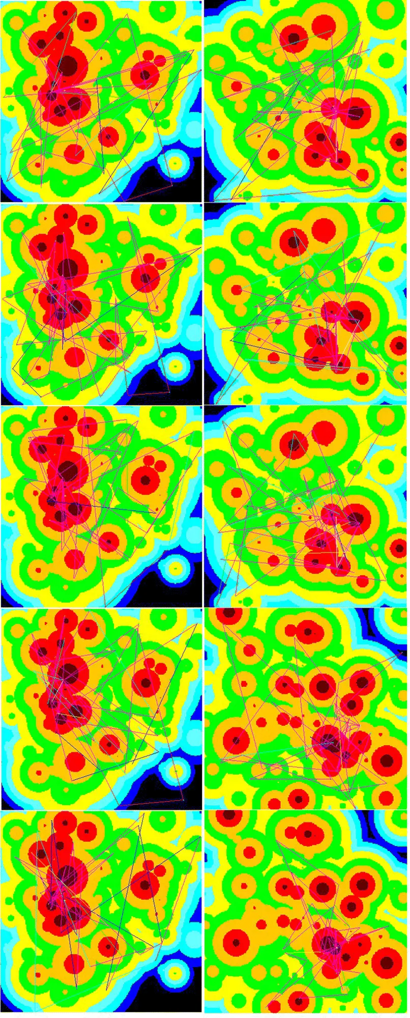
Figure 2.10 Five steps of the static (left) and dynamic (right) landscape networks.

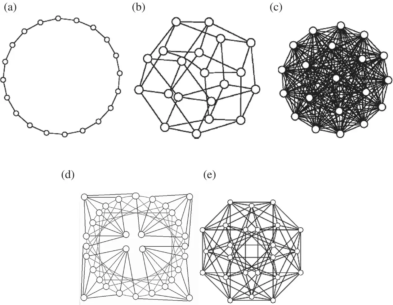
Figure 2.11 The homogeneous topologies. (a) Ring topology, (b) square topology, (c) global topology, (d) hexagon topology, and (e) octagon topology.

Meanwhile in the dynamic landscape, it is possible to see in Figure 2.10. that they are just beginning to cluster as the agents in the static landscape did, when the first dynamic change occurs to the landscape. The agent cluster, which had previously begun congregating on the overall maximum for the dynamic landscape, is suddenly clustered near a new overall maximum, although the centroid of the cluster is not on it. But because the loosely clustered group was near the overall maximum, they were able to then cluster on the maximum and send out exploratory agents to investigate the newly changed landscape. As the A ‐value for the dynamic landscape is 3.5, this means that each dynamic shift will be a radical update which can result in the total possible maximum being significantly lower as no cone approaches a height similar to those of a pre‐updated landscape. This will be displayed later in the scoring results of the agents working in the static and dynamic landscapes.

The movement of the social clusters, with regards to the network topologies displayed in Figure 2.11, gives us an idea of how the mass of agents moves, with new, more rewarding locations, being disseminated among the other agents at varying rates depending on the shape of the network topology. As the network change will not only produce new information but will make some old information obsolete. For example, overabundance of connections may be both beneficial and detrimental depending on which information is discovered first. Therefore, any poisonous data introduced into a network can take longer to be purged from the system based on how it is able to move through said network ( Figure 2.12).

While continuing the simulation, it is possible to view not only the agents and their network shared network topology, but also the area which each influencing knowledge source encompasses. By identifying each agent with the knowledge source which is influencing it, and then compiling the coordinates of each agent, it is possible to draw a bounding box which contains all agents that adhere to a given knowledge source. The structures of these boxes and their subsequent expansions and contractions can serve to highlight the nature of each knowledge source.

Boxes that contract over successive steps indicate an exploitative knowledge source, such as the Situational knowledge source. These knowledge sources will tend to focus on a known best example and explore in its immediate vicinity for any possible improvement. Boxes that expand over successive steps or trend toward more encompassing sizes typically represent the explorative knowledge sources, such as the Topographical knowledge source. These knowledge sources tend to send out agents to possibly high‐scoring predicted spots based on calculations made with known data.

While explorative search suffers from covering massive amounts of ground with limited agents, exploitative suffers from a blindness brought on from agents that only focus on the immediate. With agents sharing information between knowledge sources, however, both types of knowledge source will benefit.

When the CAT system has finished running its generations across the two landscapes, it is possible to view the results of each generation's top scoring results. In Figure 2.13these results are depicted, with each line indicating the results of one of the knowledge sources. The static landscape's generations display a steady maintenance of the discovered maximum in the landscape, while the dynamic landscape's generations show the dramatic drop‐off each time a dynamic update of the landscape occurs.

Earlier it was mentioned that the homogeneous distribution of agents during the initialization phase of the runs gave a wide breadth of knowledge to the knowledge sources to use during each subsequent step. This could account for rapid early acquisition of a maximum. However, the dynamic landscape's violent landscape changes, which can result in clusters of agents suddenly being on a low‐scoring point in the landscape in unfamiliar terrain, show a more dramatic difference between the scores of the agents immediately after the shift, and several steps later when the maximum is reclaimed.

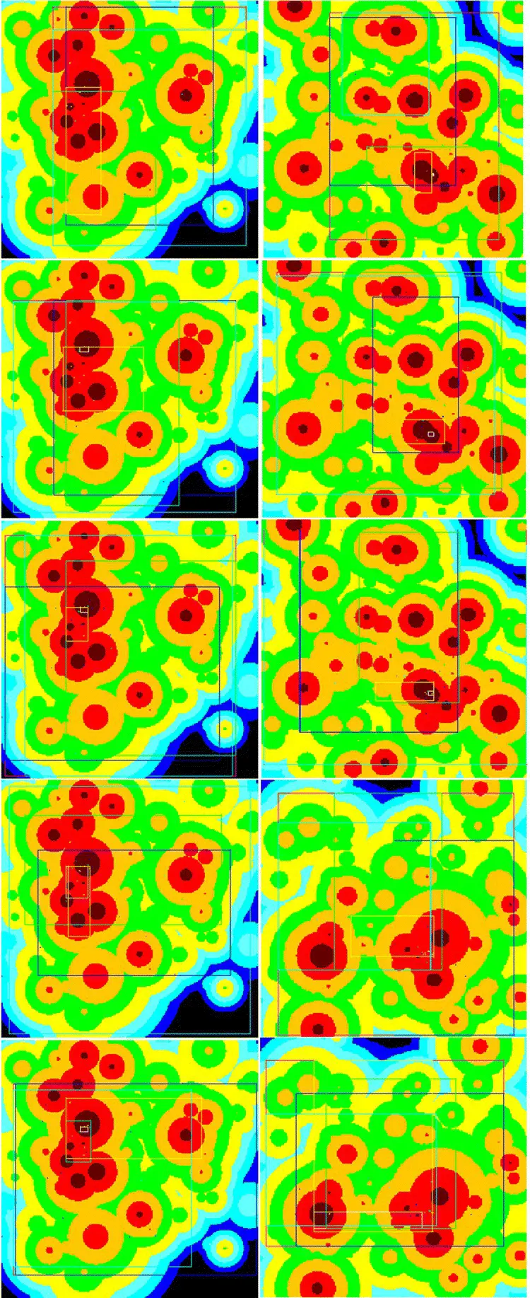
Figure 2.12 Five steps of the static (left) and dynamic (right) bounding boxes.

Also due to the chaotic nature of the 3.5 value of A of the dynamic landscape's updates, note that the overall possible maximum changes not only its position but also its magnitude with the shifts. This explains the low yet stable fitness values achieved during different points in the dynamic landscape, where plateaus occur in the data.

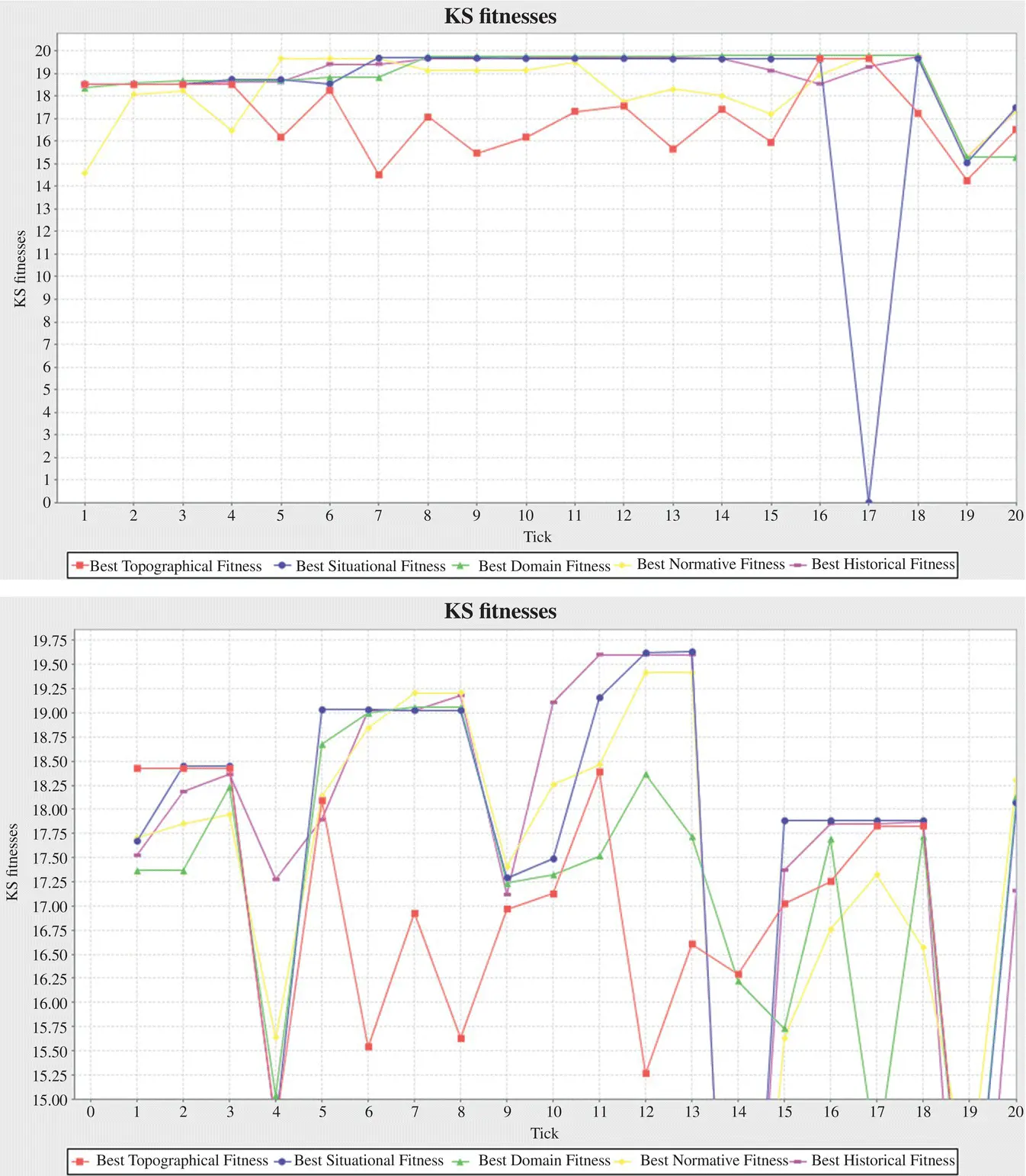
Figure 2.13 The KS fitnesses for the static (above) and dynamic (below) landscapes.

In addition, as noted in the discussion of bounding boxes, the exploitative and explorative aspects of the knowledge sources can be discerned from their adherence to a found maximum when viewed by the knowledge source fitnesses. Those exploitative knowledge sources, such as Situational and Historical, will tend to achieve a high fitness and then stay at that level. The explorative knowledges source on the other hand, such as Topographical and Domain, will tend to stay away from the maximum as they seek out more information.

In Figure 2.14, we can see the areas of each bounding box produced by each knowledge source. It can be seen in this visualization that the two most exploitative knowledge sources, situational and historical, regularly have the smallest areas of coverage, while the two most explorative knowledge sources, normative and topographical, cover the largest areas. The domain knowledge source straddles the line between these two methodologies of exploration and exploitation, expanding and contracting itself as data come in, focusing on a transitional region between the more extreme knowledge sources.