Data Analytics in Bioinformatics
Здесь есть возможность читать онлайн «Data Analytics in Bioinformatics» — ознакомительный отрывок электронной книги совершенно бесплатно, а после прочтения отрывка купить полную версию. В некоторых случаях можно слушать аудио, скачать через торрент в формате fb2 и присутствует краткое содержание. Жанр: unrecognised, на английском языке. Описание произведения, (предисловие) а так же отзывы посетителей доступны на портале библиотеки ЛибКат.
- Название:Data Analytics in Bioinformatics
- Автор:
- Жанр:
- Год:неизвестен
- ISBN:нет данных
- Рейтинг книги:5 / 5. Голосов: 1
-
Избранное:Добавить в избранное
- Отзывы:
-
Ваша оценка:
Data Analytics in Bioinformatics: краткое содержание, описание и аннотация
Предлагаем к чтению аннотацию, описание, краткое содержание или предисловие (зависит от того, что написал сам автор книги «Data Analytics in Bioinformatics»). Если вы не нашли необходимую информацию о книге — напишите в комментариях, мы постараемся отыскать её.
Data Analytics in Bioinformatics — читать онлайн ознакомительный отрывок
Ниже представлен текст книги, разбитый по страницам. Система сохранения места последней прочитанной страницы, позволяет с удобством читать онлайн бесплатно книгу «Data Analytics in Bioinformatics», без необходимости каждый раз заново искать на чём Вы остановились. Поставьте закладку, и сможете в любой момент перейти на страницу, на которой закончили чтение.
Интервал:
Закладка:
2.2 Clustering in Unsupervised Learning
Clustering is a technique through which the unlabeled dataset is being grouped based upon the similarity and the characteristics of the data from which a structured output is obtained [4]. The popular algorithms [5] of clustering include
k-means (partitions the data)
hierarchial (AGNES—agglomerative nesting)
Density-based (DBSCAN—Density based spatial clustering with noise)
Model-based (SOM—self-organizing maps)
Grid-based (STING—statistical information grid)
Soft clustering (FCM—Fuzzy Class Membership).
2.3 Clustering in Bioinformatics—Genetic Data
Clustering algorithms in bioinformatics are mostly used to decrypt the salient data in gene expression which is used to acknowledge biological processes in an organism. Gene expression exhibits divergent nature under varying clinical conditions, different tissues and different organisms. The observations drawn from the above conditions enhance the study and analysis of gene functionality. This in turn supports in drug discovery based on the diseased area and the varying nature of genes with diseased condition [28]. With the presence of voluminous amount of genes, it is complex to interpret the data. Therefore, the hidden patterns are being revealed by applying clustering techniques providing a better understanding of functioning of genes and the cellular and biological process of a cell as well [9]. Clustering can be either hard or overlapping. Contemplating every gene as a single cluster is referred as hard clustering whereas overlapping cluster is defined as degree of integration of relatable genes in diverse clusters to every gene expression [10].
2.3.1 Microarray Analysis
The exploration of genomics is centered upon the study of single genes; contrarily microarray analysis is a technology where thousands of gene expressions and its levels are identified under a microscopic slide upon which chips are placed to collect the data which in turn referred as gene chips or DNA chips [12].
In microarray analysis mRNA molecules are gathered from a reference sample (e.g. sample of diseased patient) and test sample (molecules of any individual). The data is combined using probes and if similarities are identified then they are moved into a cluster. If they are found to be dissimilar, they are moved to another cluster. Hence, the clusters are now labeled based on their similarities [12].
During the microarray analysis the data gathered from microarray images are used to construct matrices (refer to Table 2.1) in which rows hold genes and columns hold different conditions viz. different tissues, clinical condition, different biological processes. Expression level data is maintained in each cell of the matrix (refer to Table 2.1) which is uniquely numbered using every gene in every other sample.
Table 2.1Gene expression data matrix representation.
| Sample 1 | Sample 2 | Sample 3 | Sample 4 | Sample m | |
| Gene1 | C11 | C12 | C13 | C13 | C1m |
| Gene2 | C21 | C22 | C23 | C24 | C2m |
| Gene3 | C31 | C32 | C33 | C34 | C3m |
| Gene4 | C41 | C42 | C43 | C44 | C4m |
| Gene n | Cn1 | Cn2 | Cn3 | Cn4 | Cnm |
These gene expression matrices are summed up into a database as shown in Figure 2.2 which acts as a repository for all the genetic information like gene regulation, genetics functionality of diseases, drug discovery based upon gene structures, response to drug projection and so on. These databases with all the genomic information when searched for particular instance of genes, it retrieves all the relevant information with high similarities using these clustering algorithms [32].
The sequence of actions for Clustering of Gene Expression (GE), include
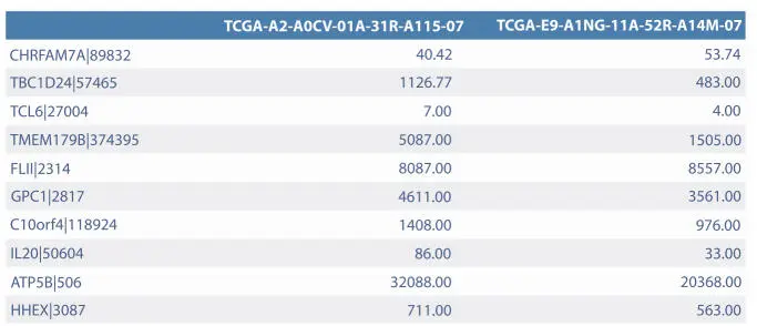
Figure 2.2Example matrix of gene expression (10 genes in a row and 2 samples in columns) [29–31].
A matrix which hold the data of GE structure which consists of size, dimension, number, origin, etc.
Features are extracted to identify the similarities (feature extraction). The input data is reduced without loss of information making it more suitable to application is called feature selection or feature reduction. The feature reduction can be achieved using few common algorithms for example Principal Component Analysis [11].
Based upon similarities or features, all the genes which express similar expression are made into one cluster and which are distinct are grouped into another cluster. The degree of similarity or the proximity levels are computed using certain distance metrics applied on gene expression data provided. Euclidean distance, Manhattan distance, Mahalanobis distance, etc. are few metrics applied to quantify the level of similarity in order to form a cluster.
2.3.2 Clustering Algorithms
The genetic data (genes) are closely connected. Based upon the dataset appropriate clustering algorithms need to be chosen. These clustering approaches also reveals about the relationship between the clusters based upon the similarity. This section explains various partition algorithms. Figure 2.3 summarizes various clustering based partitions those can be used in Bioinformatics.
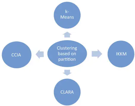
Figure 2.3Partition clustering algorithms.
2.3.3 Partition Algorithms
2.3.3.1 k-Means Clustering
This algorithm partitions the dataset of n objects into k clusters in the feature space. The value of k (number of clusters) is fixed beforehand. Initially the algorithm randomly assumes k number of cluster centers (cluster mean) in the feature space. The distance (computed using Euclidean distance) of each gene sample is computed from all these cluster means. The sample is then grouped under the cluster that has minimum distance from the sample. The same process is followed for all the samples. Once all the samples are grouped under one of these clusters, each cluster mean is computed again considering the entire samples in that cluster and the cluster mean is updated. The above steps are iterated until the algorithm forms k stable clusters.
The drawback of such algorithm is that determining the clusters (k) prior to implementation reduces the effectiveness of cluster formation and is prone to noisy data in gene expression values [13].
2.3.3.2 Cluster Center Initialization Algorithm (CCIA)
In traditional k-means algorithm the centroids of clusters are randomly selected initially, yielding low quality clusters. As an attempt in producing high quality clustering CCIA is introduced. This algorithm can be referred as an enhancement to k-means algorithm in which centroids (k) are accurately selected which are distant from the outliers. This selection process is done by computing mean and standard deviation on the data elements. CCIA now examines most nearest set of elements from the dataset (D) and fabricates into a new dataset (X) after discarding the outliers. Later those set of elements are eliminated from the dataset (D). This process is iterated until the dataset (X) equals with (k).
Читать дальшеИнтервал:
Закладка:
Похожие книги на «Data Analytics in Bioinformatics»
Представляем Вашему вниманию похожие книги на «Data Analytics in Bioinformatics» списком для выбора. Мы отобрали схожую по названию и смыслу литературу в надежде предоставить читателям больше вариантов отыскать новые, интересные, ещё непрочитанные произведения.


Обсуждение, отзывы о книге «Data Analytics in Bioinformatics» и просто собственные мнения читателей. Оставьте ваши комментарии, напишите, что Вы думаете о произведении, его смысле или главных героях. Укажите что конкретно понравилось, а что нет, и почему Вы так считаете.