Robert J. Moffat - Planning and Executing Credible Experiments

An analysis is a persistent thing. It continues to exist on paper long after the analyst lays down his or her pencil. That sheet (or that computer program) can be given to a colleague for review: “Do you see any error in this?”

An experiment is a sequence of states that exist momentarily and then are gone forever. The experimenter is a spectator, watching the event – the only trace of the experiment is the data that have been recorded. If those data don’t accurately reflect what happened, you are out of luck.

An experiment can never be repeated – you can only repeat what you think you did. Taking data from an experiment is like taking notes from a speech. If you didn't get it when it was said, you just don't have it. That means that you can never relax in the lab. Any moment when your attention wanders is likely to be the moment when the results are “unusual.” Then, you will wonder, “Did I really see that?” [Please see “Positive Consequences of the Reproducibility Crisis” ( Panel 2.1). The crisis, by way of the Ioannidis article, was mentioned in Chapter 1.]

The clock never stops ticking, and an instant in time can never be repeated. The only record of your experiment is in the data you recorded. If the results are hard to believe, you may well wish you had taken more detailed data. It is smart to analyze the data in real time, so you can see the results as they emerge. Then, when something strange happens in the experiment, you can immediately repeat the test point that gave you the strange result. One of the worst things you can do is to take data all day, shut down the rig, and then reduce the data. Generally, there is no way to tell whether unusual data should be believed or not, unless you spot the anomaly immediately and can repeat the set point before the peripheral conditions change.

The experimental approach requires gathering enough input–output datasets so that the form of the model function can be determined with acceptable uncertainty. This is, at best, an approximate process, as can be seen by a simple example. Consider the differences between the analytical and the experimental approaches to the function y = sin( x ). Analytically, given that function and an input set of values of x , the corresponding values of y can be determined to within any desired accuracy, by using the known behavior of the function y = sin( x ). Consider now a “black box” which, when fed values of x , produces values of y . With what certainty can we claim that the model function (inside the box) is really y = sin( x )? Obviously, the certainty is limited by the accuracy of the input and the output. What uncertainty must we acknowledge when we claim that the model function (inside the box) is y = sin( x )? That depends on the accuracy of the input and the output data points and the number and spacing of the points. With a set of data having some specified number of significant figures in the input and the output, we can say only that the model function, “evaluated at these data points, does not differ from y = sin( x ) by more than …,” or alternatively, “ y = sin( x ) within the accuracy of this experiment, at the points measured.”

That is about all we can be sure of because our understanding of the model function can be affected by the choice of the input values. Suppose that we were unfortunate enough to have chosen a sampling rate that caused our input data points (the test rig set points) to exactly match values of n π with n being an integer. Then all of the outputs would be zero, and we could not distinguish between the “aliased” model function y = 0 and the true model function y = sin( x ).

In general, with randomly selected values of x , the “resolution” of the experiment is limited by the accuracy of the input and output data. Consider Figure 2.2. In this case, sin( x ) may be indistinguishable from {sin( x ) + 0.1 sin (10 x )} if there is significant scatter in the data. In many cases, the scatter in data is, in reality, the trace of an unrecognized component of the model function that could be included. One of an experimenter's most challenging tasks is to interpret correctly small changes in the data: is this just “scatter,” or is the process trying to show me something?

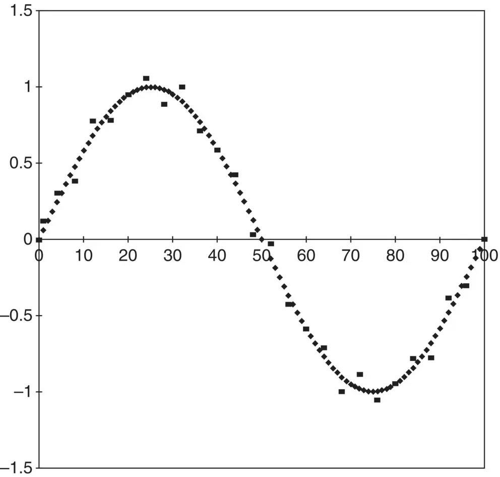
Figure 2.2 Is this a single sine wave with some scatter in the data? Does it have a superposed signal or both signal and scatter?

Another difference between experiment and analysis that is important is their description in terms of “dimensionality.” A necessary initial step in an analysis is to set the dimensional domain of relevant factors; e.g. y = f ( x 1, x 2, x 3, …, x N). Once an analyst has declared the domain, then the analyst may proceed with certainty by applying the rules appropriate for functions of N variables.

Experimentalists cannot make their results insensitive to “other factors” simply by declaration, as the analyst can. The test program must be designed to reveal and measure the sensitivity of the results to changes in the secondary variables.

Experiments are always conducted in a space of unknown dimensionality. Any variable which affects the outcome of the experiment is a “dimension” of that experiment. Whether or not we recognize the effect of a variable on the result may depend on the precision of the measurements. Thus, the number of significant dimensions for most experiments depends on the precision of the measurements of input and output and the density of data points as well as on the process being studied and the factors which are being considered.

For example, one might ask: “Does the width dimension of the test channel affect the measured value of the heat‐transfer coefficient h on a specimen placed in the tunnel?” This is a question about the dimensionality of the problem. The answer will depend on how accurately the heat‐transfer coefficient is being measured. If the scatter in the h ‐data is ±25%, then only when the blockage is high will the tunnel dimensions be important. If the scatter in h is ±1%, then the tunnel width may affect the measured value even if the blockage is as low as 2 or 3%.

One common approach to limit dimensionality of an experiment is to carefully describe the apparatus, so it could be duplicated if necessary, and then run the tests by holding constant as many variables as possible while changing the independent variables, one at a time. This is not the wisest approach. A one‐at‐a‐time experiment measures the partial derivative of the outcome with respect to each of the independent variables, holding constant the values of the secondary variables. Although this seems to limit dimensionality, it does not. Running only a partial derivative experiment begs the question of sensitivity to peripheral factors: that is, holding the interaction effect constant does not make it go away, it simply makes it more difficult to find.

Wiser approaches are discussed in Chapters 8 and 9, whereby systematic investigation of the sensitivity of the results to the details of the technique and the equipment helps the dimensionality of the experiment to be known. Whatever remains unknown contributes to experimental uncertainty.