James W. Gregory - Introduction to Flight Testing
Здесь есть возможность читать онлайн «James W. Gregory - Introduction to Flight Testing» — ознакомительный отрывок электронной книги совершенно бесплатно, а после прочтения отрывка купить полную версию. В некоторых случаях можно слушать аудио, скачать через торрент в формате fb2 и присутствует краткое содержание. Жанр: unrecognised, на английском языке. Описание произведения, (предисловие) а так же отзывы посетителей доступны на портале библиотеки ЛибКат.
- Название:Introduction to Flight Testing
- Автор:
- Жанр:
- Год:неизвестен
- ISBN:нет данных
- Рейтинг книги:3 / 5. Голосов: 1
-
Избранное:Добавить в избранное
- Отзывы:
-
Ваша оценка:
Introduction to Flight Testing: краткое содержание, описание и аннотация
Предлагаем к чтению аннотацию, описание, краткое содержание или предисловие (зависит от того, что написал сам автор книги «Introduction to Flight Testing»). Если вы не нашли необходимую информацию о книге — напишите в комментариях, мы постараемся отыскать её.
Introduction to Flight Testing
Key features:
Provides an introduction to the basic flight testing methods and instrumentation employed on general aviation aircraft and unmanned aerial vehicles.
Includes examples of flight testing on general aviation aircraft such as Cirrus, Diamond, and Cessna aircraft, along with unmanned aircraft vehicles.
Suitable for courses on Aircraft Flight Test Engineering. Provides an introduction to the basic flight testing methods employed on general aviation aircraft and unmanned aerial vehicles
Introduction to Flight Testing
Introduction to Flight Testing
Introduction to Flight Testing — читать онлайн ознакомительный отрывок
Ниже представлен текст книги, разбитый по страницам. Система сохранения места последней прочитанной страницы, позволяет с удобством читать онлайн бесплатно книгу «Introduction to Flight Testing», без необходимости каждый раз заново искать на чём Вы остановились. Поставьте закладку, и сможете в любой момент перейти на страницу, на которой закончили чтение.
Интервал:
Закладка:
Despite the fact that gravity varies with altitude, it is convenient to derive the standard atmosphere based on the assumption of constant gravitational acceleration. In order to do so, we must define a new altitude, the geopotential altitude, h , which we will use in the hydrostatic equation with the assumption of constant gravity. Referring to Eq. (2.3), we can also write the hydrostatic equation as a function of geopotential altitude and constant gravitational acceleration,
(2.5) 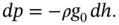
Taking the ratio of (2.5)and (2.3), we have
(2.6) 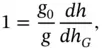
since the differential pressure and density terms cancel out for a given change of pressure. The small difference between g 0and g then leads to a small difference between the geopotential and geometric altitudes. Combining Eqs. (2.4)and (2.6)produces
(2.7) 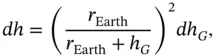
which can be integrated between sea level and an arbitrary altitude to find
(2.8) 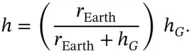
This expression defines the relationship between geopotential altitude, h , and geometric altitude, h G, which can also be solved for geometric altitude,
(2.9) 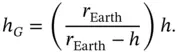
In our derivation of the standard atmosphere, we will use geopotential altitude, h , and assume constant g 0. Properties of the standard atmosphere such as temperature, pressure, and density, i.e., ( T , p , ρ ), will be found as a function of geopotential altitude, h , and then mapped back to geometric altitude, h G, by Eq. (2.9). In this work, we are focused on the lower portions of the atmosphere where most aircraft fly ( h ≤ 20 km or 65, 617 ft). At that upper altitude limit, Eq. (2.9)predicts a maximum difference of 0.31% between the geometric and geopotential altitude. Thus, in many cases related to flight testing, this difference between geopotential and geometric altitudes can be neglected.
2.2.3 Temperature
Temperature at any given point in the Earth's atmosphere will depend not only on the altitude but also on time of year, latitude, and local weather conditions. Since the variation of temperature has spatial, temporal, and stochastic input, the development of the standard atmosphere as a function of only altitude inherently involves many approximations. Thus, we might anticipate that the actual temperature at a given location can deviate significantly from the standard value.
The standard temperature profile has been determined through an average of significant amounts of data from sounding balloons launched multiple times a day over a period of many years, at locations around the globe. The resulting temperature profile is a function of geopotential altitude, with the lapse rate, a = dT / dh , representing the linear variation of temperature with altitude for each region (see Table 2.1and Figure 2.3). In the troposphere (0 ≤ h ≤ 11 km), the standard temperature lapse rate is defined as −6.5 K/km, starting at T SL= 288.15 K. In the lower portion of the stratosphere (11 < h ≤ 20 km), the temperature is presumed to be constant at 216.65 K. Starting at 20 km, the temperature then increases at a rate of 1 K/km due to ozone heating of the upper stratosphere. Based on the data in Table 2.1, we can write expressions for the temperature profile throughout the standard atmosphere as
(2.10) 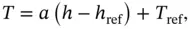
where “ref” refers to the base of the layer (defined by either sea level conditions, or the top of the prior atmospheric layer, working upwards). Output from Eq. (2.10)can be stacked for each altitude layer, one on top of another, to define the entire standard temperature profile. Since most flight testing, especially for light aircraft and drones, occurs at altitudes below 20 km, we will focus our attention on the troposphere and lower portion of the stratosphere.
Table 2.1 Definition of temperature lapse rates in various regions of the atmosphere.
Source: Data from NOAA et al. 1976.
| Region | h 1(km) | h 2(km) | a = dT / dh (K/km) |
|---|---|---|---|
| Troposphere | 0 | 11 | −6.5 |
| Stratosphere | 11 | 20 | 0.0 |
| 20 | 32 | 1.0 | |
| 32 | 47 | 2.8 | |
| 47 | 51 | 0.0 | |
| Mesosphere | 51 | 71 | −2.8 |
| 71 | 84.852 | −2.0 |
h 1and h 2are the beginning and ending altitudes of each region, respectively.
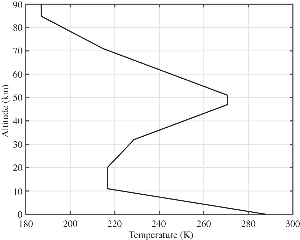
Figure 2.3 Standard temperature profile.
2.2.4 Viscosity
We also need to define an expression for dynamic viscosity, μ , which depends on temperature. The most significant impact of viscosity is in the definition of Reynolds number,
(2.11) 
which is an expression of the ratio of inertial to viscous forces (here, U ∞is the freestream velocity or airspeed, and c is the mean aerodynamic chord of the wing). Reynolds number has a significant impact on boundary layer development and aerodynamic stall, as we will see in Chapter 12.
The viscosity of air is related to the rate of molecular diffusion, which is a function of temperature (Sutherland 1893). This relationship has been distilled down to Sutherland's Law,
(2.12) 
where T is the temperature in absolute units, and β and S viscare empirical constants, provided in Table 2.2for both English and SI units (NOAA et al. 1976). Based on Eq. (2.12), the viscosity of a gas increases with increasing temperature. Thus, the dynamic viscosity decreases gradually through the troposphere, starting with the standard sea level value of μ SL= 1.7894 × 10 −5kg/(s m) = 3.7372 × 10 −7slug/(s ft) at a temperature of T SL= 288.15 K = 518.67 ° R. If kinematic viscosity ( ν ) is desired instead of dynamic viscosity, it can be found based on its definition,
(2.13) 
Интервал:
Закладка:
Похожие книги на «Introduction to Flight Testing»
Представляем Вашему вниманию похожие книги на «Introduction to Flight Testing» списком для выбора. Мы отобрали схожую по названию и смыслу литературу в надежде предоставить читателям больше вариантов отыскать новые, интересные, ещё непрочитанные произведения.


Обсуждение, отзывы о книге «Introduction to Flight Testing» и просто собственные мнения читателей. Оставьте ваши комментарии, напишите, что Вы думаете о произведении, его смысле или главных героях. Укажите что конкретно понравилось, а что нет, и почему Вы так считаете.