Giuseppe A. Paleologo - Advanced Portfolio Management
Здесь есть возможность читать онлайн «Giuseppe A. Paleologo - Advanced Portfolio Management» — ознакомительный отрывок электронной книги совершенно бесплатно, а после прочтения отрывка купить полную версию. В некоторых случаях можно слушать аудио, скачать через торрент в формате fb2 и присутствует краткое содержание. Жанр: unrecognised, на английском языке. Описание произведения, (предисловие) а так же отзывы посетителей доступны на портале библиотеки ЛибКат.
- Название:Advanced Portfolio Management
- Автор:
- Жанр:
- Год:неизвестен
- ISBN:нет данных
- Рейтинг книги:3 / 5. Голосов: 1
-
Избранное:Добавить в избранное
- Отзывы:
-
Ваша оценка:
Advanced Portfolio Management: краткое содержание, описание и аннотация
Предлагаем к чтению аннотацию, описание, краткое содержание или предисловие (зависит от того, что написал сам автор книги «Advanced Portfolio Management»). Если вы не нашли необходимую информацию о книге — напишите в комментариях, мы постараемся отыскать её.
Advanced Portfolio Management
You will learn how to:
Separate stock-specific return drivers from the investment environment’s return drivers Understand current investment themes Size your cash positions based on Your investment ideas Understand your performance Measure and decompose risk Hedge the risk you don’t want Use diversification to your advantage Manage losses and control tail risk Set your leverage Author Giuseppe A. Paleologo has consulted, collaborated, taught, and drank strong wine with some of the best stock-pickers in the world; he has traded tens of billions of dollars hedging and optimizing their books and has helped them navigate through big drawdowns and even bigger recoveries. Whether or not you have access to risk models or advanced mathematical background, you will benefit from the techniques and the insights contained in the book—and won't find them covered anywhere else.
Advanced Portfolio Management — читать онлайн ознакомительный отрывок
Ниже представлен текст книги, разбитый по страницам. Система сохранения места последней прочитанной страницы, позволяет с удобством читать онлайн бесплатно книгу «Advanced Portfolio Management», без необходимости каждый раз заново искать на чём Вы остановились. Поставьте закладку, и сможете в любой момент перейти на страницу, на которой закончили чтение.
Интервал:
Закладка:
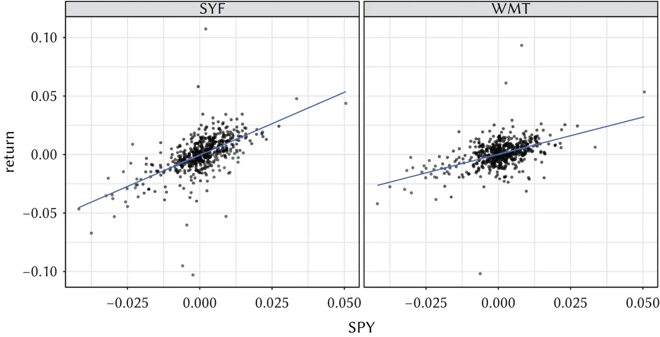
Figure 3.1 Linear regression of Synchrony's (SYF) and Wal-Mart's (WMT) daily returns against the SPY daily returns, using daily returns for the years 2018 and 2019.
3.2 Alpha and Beta
Consider the regression line for SYF again. The complete formula for a linear regression includes an intercept and an error term, or residual. We write this explicitly. For a given stock,
(3.1) 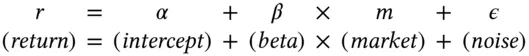
Visually, this relationship is shown in Figure 3.2. We already introduced the term  . This market component of the stock return is also called the systematic return of a stock. The first term on the left is the intercept
  ; it is a constant. When the market return is zero, the daily stock return is in expectation equal to alpha. No one observes expected returns, however. Even in the absence of market returns, the realized return of the stock would be
  . The last term is the “noise” around the stock return; it is also called idiosyncratic return of the stock. The terms specific and residual are also common, and we use all of them interchangeably. We would like to believe that this nuisance term is specific to the company: every commonality among the stocks comes the beta and the market return. The simple model of Equation (3.1), with a single systematic source of return for all the stocks, is called a single-factor model .
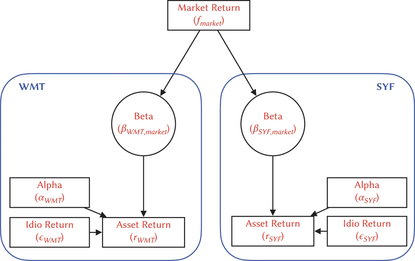
Figure 3.2 Flowchart illustrating the relationships between market, idio and asset returns, mediated by betas and offset by alphas. Market return times beta is added to alpha and idiosyncratic return to yield the total return.
The term  is only dependent on the company and nothing else. If that is the case, then the nuisance of many stocks diversifies away, a phenomenon that we will revisit many times in the following chapters. Alpha is the expected value of idiosyncratic return, and
  is the noise masking it. So, if we take the expectation of a stock return, what do we get? Alpha and Beta are constant, epsilon has expectation equal to zero, and the market return has a non-zero return.

There is general agreement that accurately forecasting market returns is very difficult, and it is, at the very least, not in the mandate of a fundamental analyst. A macroeconomic investor may have an edge in forecasting the market; a fundamental one typically does not have a differentiated view. We can sketch the roles of various investment professionals as follows:
To estimate as accurately as possible is the job of the fundamental investor.
To estimate , identify the correct benchmarks , and the returns is the job of the quantitative risk manager.
To estimate the expected value of (especially if the expectation changes over time) is the job of the macroeconomic investor.
But ultimately it is the job of the portfolio manager – who combines knowledge about mispricing with portfolio construction – to make use of relationship (3.1)to her own advantage.
3.3 Where Does Alpha Come From?
In the previous sections we used the example of SYF and WMT. We now analyze in more detail the historical estimates for SYF, using returns for year 2018. Table 3.1shows the estimates and the 95% confidence interval. The error around the alpha estimate is much larger than the estimate itself, which is not the case for beta. Table 3.2shows the high degree of variability in the alphas, whereas the betas are relatively stable. This is the case for most stocks: estimates of alphas have large associated confidence intervals, and they seem to vary over time. You can't observe alpha directly, and you cannot estimate it easily from time series of returns. It is the job of the fundamental analyst to predict forward-looking alpha values based on deep fundamental research. The ability to combine these alpha forecasts in non-trivial ways from a variety of sources and to process a large number of unstructured data is a competitive advantage of fundamental investing, and one that will not go away soon . We list some of data sources and processes involved in the alpha generation process.
Table 3.1 Parameter estimates for Synchrony's returns regressed against SP500 returns, 2018. Alphas are expressed in percentage annualized returns.
| Parameter | Estimate | 95% conf.interval |
|---|---|---|
| alpha (%) | −24 | (−88, +8) |
| beta | 1.02 | (0.84, 1.20) |
Table 3.2 Parameter estimates for Synchrony's returns regressed against SP500 returns, 2015–2019. Alphas are expressed in percentage annualized returns.
| Year | Alpha (%) | Beta |
|---|---|---|
| 2016 | 6 | 1.45 |
| 2017 | −24 | 1.79 |
| 2018 | −40 | 1.02 |
| 2019 | 16 | 1.15 |
| 2020 | −19 | 1.69 |
Valuation Analysis. This differentiated view comes from a company business model whose data are coming primarily from Cash Flow Statements, Balance Sheets (Statements of Financial Positions), Income Statements and Stakeholder Equity Statements. It is complemented by macroeconomic data affecting the production function of the company as well as demand for its products and services. This is the domain of fundamental analysis [T. Koller and Wessels, 2015] and affects both short-term forecasts, e.g., earnings or the event of a sell-side analyst downgrading or upgrading a recommendation, and long-term forecast, such as the potential long-term unsuitability of a business.
Alternative Data. Enabled by the availability of transactional data (e.g., credit card transactions) and environmental data (such as satellite imaging), these data complement fundamental analysis and give short-term information about demand, supply, costs, and potential risks. A textbook account of alternative data in finance is [Denev and Amin, 2020]; a reference for data sources, published by J.P. Morgan, is [Kolanovic and Krishnamachari, 2017].
Sentiment Analysis. This can be interpreted as the subset of alternative data that gives information about demand that is a function of the consumer's expectations of the future state of the economy. Common macroeconomic time series are Conference Board's Consumer Confidence Index, the University of Michigan's Survey of Consumers, and the Purchasing Managers' Index. At the company level, it is possible to gain information from unstructured data [Loughran and McDonald, 2016].
Читать дальшеИнтервал:
Закладка:
Похожие книги на «Advanced Portfolio Management»
Представляем Вашему вниманию похожие книги на «Advanced Portfolio Management» списком для выбора. Мы отобрали схожую по названию и смыслу литературу в надежде предоставить читателям больше вариантов отыскать новые, интересные, ещё непрочитанные произведения.


Обсуждение, отзывы о книге «Advanced Portfolio Management» и просто собственные мнения читателей. Оставьте ваши комментарии, напишите, что Вы думаете о произведении, его смысле или главных героях. Укажите что конкретно понравилось, а что нет, и почему Вы так считаете.