Ian Smith - Smith's Elements of Soil Mechanics
Здесь есть возможность читать онлайн «Ian Smith - Smith's Elements of Soil Mechanics» — ознакомительный отрывок электронной книги совершенно бесплатно, а после прочтения отрывка купить полную версию. В некоторых случаях можно слушать аудио, скачать через торрент в формате fb2 и присутствует краткое содержание. Жанр: unrecognised, на английском языке. Описание произведения, (предисловие) а так же отзывы посетителей доступны на портале библиотеки ЛибКат.

- Название:Smith's Elements of Soil Mechanics
- Автор:
- Жанр:
- Год:неизвестен
- ISBN:нет данных
- Рейтинг книги:5 / 5. Голосов: 1
-
Избранное:Добавить в избранное
- Отзывы:
-
Ваша оценка:
Smith's Elements of Soil Mechanics: краткое содержание, описание и аннотация
Предлагаем к чтению аннотацию, описание, краткое содержание или предисловие (зависит от того, что написал сам автор книги «Smith's Elements of Soil Mechanics»). Если вы не нашли необходимую информацию о книге — напишите в комментариях, мы постараемся отыскать её.
Smith's Elements of Soil Mechanics — читать онлайн ознакомительный отрывок
Ниже представлен текст книги, разбитый по страницам. Система сохранения места последней прочитанной страницы, позволяет с удобством читать онлайн бесплатно книгу «Smith's Elements of Soil Mechanics», без необходимости каждый раз заново искать на чём Вы остановились. Поставьте закладку, и сможете в любой момент перейти на страницу, на которой закончили чтение.
Интервал:
Закладка:
The smallest aperture generally used in soils work is that of the 0.063 mm size sieve. Below this size (i.e. silt and clay sizes) the distribution curve must be obtained by sedimentation (following either a pipette or hydrometer method of analysis). Unless a centrifuge is used, it is not possible to determine the range of clay sizes in a soil, and usually it is adequate to just obtain the total percentage of clay sizes present. The procedures for sieve, pipette and hydrometer analyses are given in BS EN ISO 17892‐4:2016 (BSI, 2016).
Examples of particle size distribution, or grading , curves for different soil types are shown in Fig. 1.10. From these grading curves it is possible to determine for each soil, the total percentage of a particular size, and the percentage of particle sizes larger or smaller than any particular particle size.
The effective size of a distribution, D10
An important particle size within a soil distribution is the effective size , which is the largest size of the smallest 10%. It is given the symbol D 10. Other particle sizes, such as D 30and D 60, are defined in the same manner.
Grading of a distribution
For a granular soil, the shape of its grading curve indicates the distribution of the soil particles within it.
If the shape of the curve is not too steep and is more or less constant over the full range of the soil's particle sizes, then the particle size distribution extends evenly over the range of the particle sizes within the soil and there is no deficiency or excess of any particular particle size. Such a soil is said to be well graded .
If the soil has any other form of distribution curve, then it is said to be poorly graded . According to their distribution curves, there are two types of poorly graded soil:
if the major part of the curve is steep, then the soil has a particle size distribution extending over a limited range with most particles tending to be about the same size. The soil is said to be closely graded or, more commonly, uniformly graded;
if a soil has large percentages of its bigger and smaller particles and only a small percentage of the intermediate sizes, then its grading curve will exhibit a significantly flat section or plateau. Such a soil is said to be gap graded.
The uniformity coefficient Cu and the coefficient of curvature, Cc
The grading of a soil is best determined by direct observation of its particle size distribution curve. This can be difficult for those studying the subject for the first time, but some guidance can be obtained by the use of a grading parameter known as the uniformity coefficient or by the coefficient of curvature .
(1.2) 
(1.3) 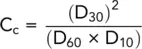
The shape of the grading of the soil can then be established through the guidance given in Table 1.2.
Other statistical data can also be obtained from the psd;
e.g. median – size at which 50% of sample is finer, D50.
Table 1.2 Shape of grading curve.
| Term | C u | C c |
|---|---|---|
| Uniformly graded | <3 | <1 |
| Poorly graded | 3–6 | <1 |
| Medium graded | 6–15 | <1 |
| Well graded | >15 | 1–3 |
| Gap graded | >15 | <0.5 |
Example 1.2Particle size distribution
The results of a sieve analysis on a soil sample were:
| Sieve size (mm) | Mass retained (g) |
| 10 | 0 |
| 6.3 | 5.5 |
| 2 | 25.7 |
| 1 | 23.1 |
| 0.600 | 22.0 |
| 0.300 | 17.3 |
| 0.150 | 12.7 |
| 0.063 | 6.9 |
2.3 g passed through the 63 μm sieve.
Plot the particle size distribution curve and determine the uniformity coefficient of the soil.
Solution:
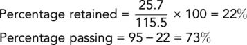
The aim is to determine the percentage of soil (by mass) passing through each sieve. To do this, the percentage retained on each sieve is determined and subtracted from the percentage passing through the previous sieve. This gives the percentage passing through the current sieve.
Calculations may be set out as follows:
| Sieve size (mm) | Mass retained (g) | Percentage retained | Percentage passing |
| 10 | 0 | 0 | 100 |
| 6.3 | 5.5 | 5 | 95 |
| 2 | 25.7 | 22 | 73 |
| 1 | 23.1 | 20 | 53 |
| 0.600 | 22.0 | 19 | 34 |
| 0.300 | 17.3 | 15 | 19 |
| 0.150 | 12.7 | 11 | 8 |
| 0.063 | 6.9 | 6 | 2 |
| Pass 0.063 | 2.3 | 2 | |
| ∑115.5 g |
e.g. 2 mm sieve:
The particle size distribution curve is shown in Fig. 1.3. Using the vertical axis, we can easily see that the soil has approximate proportions of 30% gravel and 70% sand.
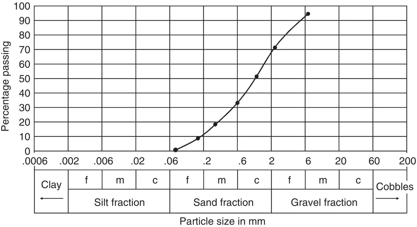
Fig. 1.3 Example 1.2.

It is also seen that the grading curve has a regular slope and therefore contains roughly equal percentages of particle sizes. The soil is a medium graded, gravelly SAND.
1.5.4 Sedimentation analysis
The fraction of soil smaller than 0.06 mm cannot be separated by sieves, so a sedimentation analysis is used to establish the proportions of silt and clay fractions. The procedure is only considered necessary if more than 10% of the soil passes the 63 μm sieve. In the test, a sample of the dry soil passing the 63 μm sieve is placed into suspension with water in a sedimentation cylinder and allowed to settle over a period of time. Measurements of the percentage of particles remaining in suspension at set time intervals are established by either using a pipette or a hydrometer. Details of the test procedures are given in BE EN ISO 17892‐4:2016 and Head (2006). The pipette procedure is described below.

Fig. 1.4 Pipette analysis arrangement.
The dry soil of known mass is placed into a sedimentation cylinder of volume 500 ml and distilled water, containing a small amount of dispersing agent, is added. A dispersing procedure (e.g. end over end shaking) is adopted to separate all the particles in the suspension. The test begins by placing the upright cylinder into a water bath at 25 °C and a stopwatch is started. Three separate sampling dips are made at a depth of 100 mm using the pipette ( Fig. 1.4) at pre‐determined times. Different particle sizes will be captured in each sample, since the larger particles fall to the bottom of the cylinder before the smaller ones.
Читать дальшеИнтервал:
Закладка:
Похожие книги на «Smith's Elements of Soil Mechanics»
Представляем Вашему вниманию похожие книги на «Smith's Elements of Soil Mechanics» списком для выбора. Мы отобрали схожую по названию и смыслу литературу в надежде предоставить читателям больше вариантов отыскать новые, интересные, ещё непрочитанные произведения.


Обсуждение, отзывы о книге «Smith's Elements of Soil Mechanics» и просто собственные мнения читателей. Оставьте ваши комментарии, напишите, что Вы думаете о произведении, его смысле или главных героях. Укажите что конкретно понравилось, а что нет, и почему Вы так считаете.