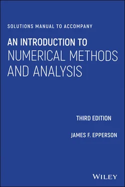
James F. Epperson - Solutions Manual to Accompany An Introduction to Numerical Methods and Analysis

11 12. What is the machine epsilon for a computer that uses binary arithmetic, 24 bits for the fraction, and rounds? What if it chops?Solution: Recall that the machine epsilon is the largest number such that the computer returns . We therefore need to find the largest number that can be represented with 24 binary digits such that , when rounded to 24 bits, is still equal to 1. This is perhaps best done by explicitly writing out the addition in binary notation. We haveIf the machine chops, then we can set all of the values to 1 and the computer will still return ; if the machine rounds, then we need to make the first digit a zero. Thus, the desired values areand

12 13. What is the machine epsilon for a computer that uses octal (base 8) arithmetic, assuming it retains 8 octol digits in the fraction?

(No exercises in this section.)

(No exercises in this section.)

1 Write each of the following polynomials in nested form.;;;.Solution:;;;.

2 Write each of the following polynomials in nested form, but this time take advantage of the fact that they involve only even powers of to minimize the computations.;.

3 Write each of the following polynomials in nested form.;;.Solution:;;.

4 Write a computer code that takes a polynomial, defined by its coefficients, and evaluates that polynomial and its first derivative using Horner's rule. Test this code by applying it to each of the polynomials in Problem 1.Solution: The following is a MATLAB script which does the assigned task, using the less efficient approach to computing the derivative.function [y, yp] = horner1(a,x) n = length(a); y = a(n); for k=(n-1):(-1):1 y = a(k) + y*x; end % yp = (n-1)*a(n); for k=(n-1):(-1):2 yp = (k-1)*a(k) + yp*x; end

5 Repeat the above, using the polynomials in Problem 2 as the test set.Solution: The same script can be used, of course.

6 Repeat the above, using the polynomials in Problem 3 as the test set.

7 Consider the polynomialThis can be written in “nested‐like” form by factoring out each binomial term as far as it will go, thus:Write each of the following polynomials in this kind of nested form.;;.Solution:;.

8 Write a computer code that computes polynomial values using the kind of nested form used in the previous problem, and test it on each of the polynomials in that problem.

9 Write a computer code to do Horner's rule on a polynomial defined by its coefficients. Test it out by using the polynomials in the previous problems. Verify that the same values are obtained when Horner's rule is used as when a naive evaluation is done.

10 Write out the Taylor polynomial of degree 5 for approximating the exponential function, using , using the Horner form. Repeat for the degree 5 Taylor approximation to the sine function. (Be sure to take advantage of the fact that the Taylor expansion to the sine uses only odd powers.)Solution: For the exponential function, we getfor the sine function we get

11 For each function in Problem 11 of §1.1, write the polynomial approximation in Horner form, and use this as the basis for a computer program that approximates the function. Compare the accuracy you actually achieve (based on the built‐in intrinsic functions on your computer) to that which was theoretically established. Be sure to check that the required accuracy is achieved over the entire interval in question.

12 Repeat the above, except this time compare the accuracy of the derivative approximation constructed by taking the derivative of the approximating polynomial. Be sure to use the derivative form of Horner's rule to evaluate the polynomial.

1 Use the methods of this section to show thatSolution: We have, for any , thatTherefore, taking ,

2 Compute, by hand, approximations to for each of the following functions, using and each of the derivative approximations contained in (2.1) and (2.5).;;;;.

3 Write a computer program which uses the same derivative approximations as in the previous problem to approximate the first derivative at for each of the following functions, using . Verify that the predicted theoretical accuracy is obtained.;;;;.Solution: I wrote a simple FORTRAN program to do this for the single case of (b). The results I got, using double precision, are in Table 2.1.Note that the error goes down by a factor of 2 for , and a factor of 4 for , thus confirming the theoretical accuracy.

4 Use the approximations from this section to fill in approximations to the missing values in Table 2.2(Table 2.4 in the text). Table 2.1Derivative Approximations.ErrorRatioErrorRatio40.442628880.0000.505108550.00080.470046581.9150.501295953.942160.484700161.9580.500325143.986320.492268861.9790.500081363.996640.496114091.9900.500020343.9991280.498051961.9950.500005094.0002560.499024711.9970.500001274.0005120.499512041.9990.500000324.00010240.499755941.9990.500000084.000 Table 2.2Table for Problem 4.1.001.00000000001.100.95135076991.200.91816874241.300.89747069631.400.88726381751.500.88622692551.600.89351534931.700.90863873291.800.93138377101.900.96176583192.001.0000000000

5 Use the error estimate (2.5) for the centered difference approximation to the first derivative to prove that this approximation will be exact for any quadratic polynomial.Solution: We have thatfor some between and . If is a quadratic, then it has the general formfor given constants , , and . But the third derivative of this kind of function will always be identically zero.

6 Find coefficients , , and so that;.Hint: Use Taylor's theorem.Solution: Write out Taylor expansions for and , thus:andMultiply the first one by 4, and subtract the two of them, to getsolve this for to getso that , , and . A similar approach works for (b), with , , and .

7 Fill in the data from Problem 4 using methods that are at each point. Hint: See the previous problem.

8 Use Taylor's Theorem to show that the approximationis .Solution: We haveandTherefore,andHence,so that, solving for , we get the desired result.

9 Use the derivative approximation from Problem 8 to approximate for the same functions as in Problem 3. Verify that the expected rate of decrease is observed for the error.

10 Use the derivative approximation from Problem 8 to fill in as much as possible of the table in Problem 4.Solution: Because this formula uses more points that are farther from the point of interest than did the previous formulas, we cannot do as much of the table as before. We get:

11 Let . Use the derivative approximation from Problem 8 to approximate using . Try to take small enough that the rounding error effect begins to dominate the mathematical error. For what value of does this begin to occur? (You may have to restrict yourself to working in single precision.)

12 Use Taylor expansions for to derive an accurate approximation to using and . Provide all the details of the error estimate. Hint: Go out as far as the fourth derivative term, and then add the two expansions.Solution: We haveandso thatThus, solving for the second derivative yields

13 Let and be given, where , for . Let be some smooth function. Use Taylor expansions for and in terms of and its derivatives at in order to construct an approximation to that depends on , , and , and which is accurate. Check your work by verifying that for you get the same results as in the text.Solution: We write the two Taylor expansionsandIf we simply subtract these, the second derivative terms will not cancel out (because ), so we have to multiply the first expansion by and the second one by to getandNow subtract to getSolve for to getBecause we assumed , there is substantial simplification that we can do to getwhich is sufficient to establish the estimate for the error.