Handbook of Intelligent Computing and Optimization for Sustainable Development

1 1) Galvanic skin response or electromodal activity

2 2) Heart rate

3 3) Electroencephalogram

4 4) Eye tracking

Many accidents which occur in the production or manufacturing sector industries are mainly due to the human related factors rather than the machines. The research on the mental work load is started well before 21st century as Sweller et al . [1] in his paper described about the concept of how skill acquisition is related to the mental workload. Similar to their work, Borghini et al . [2] pursued the work of Sweller et al . [1] further and said that making skills will help in reducing the task load. From the work of these two, we can say that the mental work load depends not only on the complexity of the task but also on the skill level of the person who is doing the job. Wang et al . [3] worked on how the mental work load of a person is related to the accidents caused by performing experiments on people solving n-back tasks. Many machine learning deep learning and other generative types of algorithms are used to predict the mental work load like support vector machines [4], hidden Markov model [5], and artificial neural networks [6]. Apart from the behavioral measures like the skill set, many tried to relate the physiological measure like eye pupil diameter, fixation, and gaze [7, 8]. The results of the study have shown that how well the mental work load data can be predicted by neural networks and Bernoulli Boltzmann machines using the eye tracking data and also how well neural networks perform in these types of tasks.

We recorded the eye tracking data of student while he debug a coding related question. There are a total of seven coding questions with two types of difficulty, easy or hard, and one question with unknown difficulty. The data acquired from the eye tracker was cleaned and processed to get the required features.

The experiment took place in the Virtual Reality Lab, Department of Industrial and Systems Engineering IIT Kharagpur. The experimental process goes as follows. A student was fixed with eye tracking device and was asked to debug seven coding related questions of known difficulty. Before solving every question, the student was asked to stare at a white blank screen to get the base coordinates. In this experiment, the eye tracker recorded the student’s data of gaze coordinates, gaze direction, pupil diameter, and fixation coordinates.

The data acquired from the eye tracker was cleaned of illegal values and null values and was processed to get the following: (1) saccadic amplitude in the X and Y direction, which is the difference between the gaze and fixation in particular direction; (2) rate of change of saccadic amplitude, in the X and Y direction, which is the saccadic amplitude divided with time difference from one fixation to the other; (3) and change in the pupil diameter, which is obtained from the difference between the pupil diameter of the student captured while debugging the code and the average of the base pupil diameter, i.e., when the student is staring at the blank screen.

Here, two types of models are used:

• Artificial Neural Network

• Bernoulli’s RBM

The brain is one of the fundamental organs in our body. It consists of a biological network with neurons (neurons: fundamental unit of brain) which take inputs in the form of signals and process them and send them as output signals. Similar to this network of neurons in the brain, there is artificial neural network. Figure 1.1represents the flowchart of the study.

Figure 1.1 Flow chart of the study.

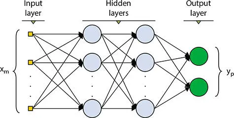
Figure 1.2 Basic neural network.

In the neural network, the neurons are arranged in multiple layers. The layer which takes the input signals is called the input layer. The signals form the Input layer are sent to hidden layers and then to the output layer. In the process of transmission from layers, weights are multiplied at every node except at the output node.

There are two techniques which standardize the weight and make ANN special; these are forward propagation and back propagation. In the normal forward propagation, simplified sample weights are multiplied at every node, and the sample outputs are recorded at the output layer. In the back propagation, as you can say from the name, it was from the output layer to the input layer. In this process, the error margin at every layer is deduced and the input weights will be changed so as to get the minimum error. The error value will be investigated every time and it is helpful in changing the weights at nodes. At every hidden node, functions called activation functions are also used. Some of them are as follows. Please see Figure 1.2.

The sigmoid function is used because it ranges between 0 and 1.

Sigmoid advantage is that it gives output which lies between 0 and 1 so we can we use it when even we need to predict the probability as probability always exists between (0, 1). There are two major disadvantages of using sigmoid activation function. One of them is that the outputs from the sigmoid are always not zero centered. The second one is the problem of gradients getting nearly 0. Please see Figure 1.3.

Tanh is quite similar to sigmoid but better and ranges from −1 to 1.

The main advantage of using tanh is that we can get outputs +ve as well as −ve which helps us to predict values which can be both +ve and −ve. The slope for the tanh graph is quite steeper than the sigmoid. Using the tanh or sigmoid totally depends on the dataset being used and the values to be predicted. Please see Figure 1.4.

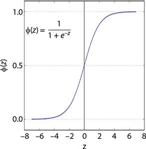
Figure 1.3 Sigmoid function.

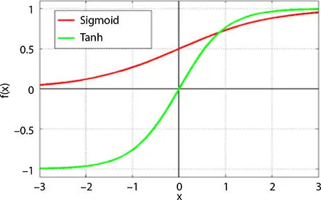
Figure 1.4 Tanh function.

ReLU ranges from 0 to infinity.

Using ReLU can rectify the vanishing grading problem. It also required very less computational power compared to the sigmoid and tanh. The main problem with the ReLU is that when the Z < 0, then the gradient tends to 0 which leads to no change in weights. So, to tackle this, ReLU is only used in hidden layers but not in input or output layers.

All these activation functions and forward and backward propagation are the key features that make artificial neural networks different from others. Please see Figure 1.5.

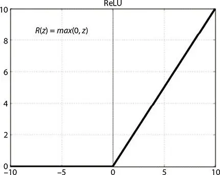
Figure 1.5 ReLU function.

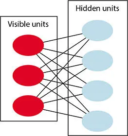
Figure 1.6 Basic Bernoulli’s restricted Boltzmann machine.