Tormod Næs - Multiblock Data Fusion in Statistics and Machine Learning
Здесь есть возможность читать онлайн «Tormod Næs - Multiblock Data Fusion in Statistics and Machine Learning» — ознакомительный отрывок электронной книги совершенно бесплатно, а после прочтения отрывка купить полную версию. В некоторых случаях можно слушать аудио, скачать через торрент в формате fb2 и присутствует краткое содержание. Жанр: unrecognised, на английском языке. Описание произведения, (предисловие) а так же отзывы посетителей доступны на портале библиотеки ЛибКат.
- Название:Multiblock Data Fusion in Statistics and Machine Learning
- Автор:
- Жанр:
- Год:неизвестен
- ISBN:нет данных
- Рейтинг книги:3 / 5. Голосов: 1
-
Избранное:Добавить в избранное
- Отзывы:
-
Ваша оценка:
Multiblock Data Fusion in Statistics and Machine Learning: краткое содержание, описание и аннотация
Предлагаем к чтению аннотацию, описание, краткое содержание или предисловие (зависит от того, что написал сам автор книги «Multiblock Data Fusion in Statistics and Machine Learning»). Если вы не нашли необходимую информацию о книге — напишите в комментариях, мы постараемся отыскать её.
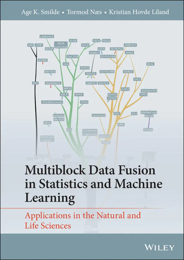
Explore the advantages and shortcomings of various forms of multiblock analysis, and the relationships between them, with this expert guide Multiblock Data Fusion in Statistics and Machine Learning: Applications in the Natural and Life Sciences
Multiblock Data Fusion in Statistics and Machine Learning: Applications in the Natural and Life Sciences
Multiblock Data Fusion in Statistics and Machine Learning — читать онлайн ознакомительный отрывок
Ниже представлен текст книги, разбитый по страницам. Система сохранения места последней прочитанной страницы, позволяет с удобством читать онлайн бесплатно книгу «Multiblock Data Fusion in Statistics and Machine Learning», без необходимости каждый раз заново искать на чём Вы остановились. Поставьте закладку, и сможете в любой момент перейти на страницу, на которой закончили чтение.
Интервал:
Закладка:
This book is an attempt to provide an up-to-date treatment of the most used and important methods within an important branch of the area; namely methods based on so-called components or latent variables. These methods have already obtained enormous attention in, for instance, chemometrics, bioinformatics, machine learning, and sensometrics and have proved to be important both for prediction and interpretation.
The book is primarily a description of methodologies, but most of the methods will be illustrated by examples from the above-mentioned areas. The book is written such that both users of the methods as well as method developers will hopefully find sections of interest. At the end of the book there is a description of a software package developed particularly for the book. This package is freely available in R and covers many of the methods discussed.
To distinguish the different types of methods from each other, the book is divided into five parts. Part I is an introduction and description of preliminary concepts. Part II is the core of the book containing the main unsupervised and supervised methods. Part III deals with more complex structures and, finally, Part IV presents alternative unsupervised and supervised methods. The book ends with Part V discussing the available software.
Our recommendations for reading the book are as follows. A minimum read of the book would involve chapters 1, 2, 3, 5, and 7. Chapters 4, 6and 8are more specialized and chapters 9and 10contain methods we think are more advanced or less obvious to use. We feel privileged to have so many friendly colleagues who were willing to spend their time on helping us to improve the book by reading separate chapters. We would like to express our thanks to: Rasmus Bro, Margriet Hendriks, Ulf Indahl, Henk Kiers, Ingrid Måge, Federico Marini, Åsmund Rinnan, Rosaria Romano, Lars Erik Solberg, Marieke Timmerman, Oliver Tomic, Johan Westerhuis, and Barry Wise. Of course, the correctness of the final text is fully our responsibility!
Age Smilde, Utrecht, The Netherlands
Tormod Næs, Ås, Norway
Kristian Hovde Liland, Ås, Norway
March 2022
List of Figures
Figure 1.1 High-level, mid-level, and low-level fusion for two input blocks.The Z’s represent the combined information from the twoblocks which is used for making the predictions. The upperfigure represents high-level fusion, where the results from two separate analyses are combined. The figure in the middle is an illustration of mid-level fusion, where components from the two data blocks are combined before further analysis. The lowerfigure illustrates low-level fusion where the data blocks are simply combined into one data block before further analysis takes place.
Figure 1.2 Idea of dimension reduction and components. The scores Tsummarise the relationships between samples; the load-ings Psummarise the relationships between variables.Sometimes weights Ware used to define the scores.
Figure 1.3 Design of the plant experiment. Numbers in the top row refer to lightlevels (in μ E m −2sec −1); numbers in the first column are degrees centigrade. Legend: D = dark, LL = low light, L = light and HL = high light.
Figure 1.4 Scores on the first two principal components of a PCA on theplant data (a) and scores on the first ASCA interaction component (b). Legend: D = dark, LL = low light, L = light and HL = high light.
Figure 1.5 Idea of copy number variation (a), methylation (b), and mutation (c)of the DNA. For (a) and (c): Source: Adapted from Koch et al., 2012.
Figure 1.6 Plot of the Raman spectra used in predicting the fat content. The dashed lines show the split of the data set into multiple blocks.
Figure 1.7 L-shape data of consumer liking studies.
Figure 1.8 Phylogeny of some multiblock methods and relationsto basic data analysis methods used in this book.
Figure 1.9 The idea of common and distinct components. Legend: blueis common variation; dark yellow and dark red are distinctvariation and shaded areas are noise (unsystematic variation).
Figure 2.1 Idea of dimension reduction and components. Sometimes W isused to define the scores T which in turn define the loadings P.
Figure 2.2 Geometry of PCA. For explanation, see text (withpermission of H.J. Ramaker, TIPb, The Netherlands).
Figure 2.3 Score (a) and loading (b) plots of a PCA on Caber-net Sauvignon wines. Source: Bro and Smilde (2014).Reproduced with permission of Royal Society of Chemistry.
Figure 2.4 PLS validated explained variance when applied to Ramanwith PUFA responses. Left: PLSR on one responseat a time. Right: PLS on both responses (standardised).
Figure 2.5 Score and loading plots for the single response PLS regression model predicting PUFA as percentage of total fat in the sample ( PUFA sample).
Figure 2.6 Raw and normalised urine NMR-spectra.Different colours are spectra of different subjects.
Figure 2.7 Numerical representations of the lengths of sticks: (a) left: the empirical relational system (ERS) of which only the length is studied, right: a numerical representation (NRS1), (b) an alternative numerical representation (NRS2) ofthe same ERS carrying essentially the same information.
Figure 2.8 Classical (a) and logistic PCA (b) on the same muta-tion data of different cancers. Source Song et al. (2017). Reproduced with permission from Oxford Academic Press.
Figure 2.9 Classical (a) and logistic PCA (b) on the same methyla-tion data of different cancers. Source Song et al. (2017). Reproduced with permission from Oxford Academic.
Figure 2.10 SCA for two data blocks; one containingbinary data and one with ratio-scaled data.
Figure 2.11 The block scores of the rows of the two blocks. Legend:green squares are block scores of the first block; blue circlesare block scores of the second block and the red stars aretheir averages (indicated with t a). Panel (a) favouring block X 1, (b) the MAXBET solution, (c) the MAXNEAR solution.
Figure 2.12 Two column-spaces each of rank two in three-dimensional space.The blue and green surfaces represent the column-spaces and the redline indicated with X 12Crepresents the common component. Source:Smilde et al. (2017). Reproduced with permission of John Wiley and Sons.
Figure 2.13 Common and distinct components. The common componentis the same in both panels. For the distinct componentsthere are now two choices regarding orthogonality: (a) bothdistinct components orthogonal to the common component, (b) distinct components mutually orthogonal. Smilde et al. (2017). Reproduced with permission of John Wiley and Sons.
Figure 2.14 Common components in case of noise: (a) maximally correlated common components within column-spaces; (b) consensus component in neither of the columns-spaces. Smilde et al. (2017). Reproduced with permission of John Wiley and Sons.
Figure 2.15 Visualisation of a response vector, y, projected ontoa two-dimensional data space spanned by x 1and x 2.
Figure 2.16 Fitted values versus residuals from a linear regression model.
Figure 2.17 Simple linear regression: ŷ = ax + b (see legend for description of elements). In addition, leverage is indi-cated below the regression plot, where leverage is at a minimum at ¯ x and increases for lower and higher x -values.
Figure 2.18 Two-variable multiple linear regression with indicated residuals and leverage (contours below regression plane).
Figure 2.19 Two component PCA score plot of concatenated Raman data.Leverage for two components is indicated by the marker size.
Читать дальшеИнтервал:
Закладка:
Похожие книги на «Multiblock Data Fusion in Statistics and Machine Learning»
Представляем Вашему вниманию похожие книги на «Multiblock Data Fusion in Statistics and Machine Learning» списком для выбора. Мы отобрали схожую по названию и смыслу литературу в надежде предоставить читателям больше вариантов отыскать новые, интересные, ещё непрочитанные произведения.


Обсуждение, отзывы о книге «Multiblock Data Fusion in Statistics and Machine Learning» и просто собственные мнения читателей. Оставьте ваши комментарии, напишите, что Вы думаете о произведении, его смысле или главных героях. Укажите что конкретно понравилось, а что нет, и почему Вы так считаете.