Tormod Næs - Multiblock Data Fusion in Statistics and Machine Learning
Здесь есть возможность читать онлайн «Tormod Næs - Multiblock Data Fusion in Statistics and Machine Learning» — ознакомительный отрывок электронной книги совершенно бесплатно, а после прочтения отрывка купить полную версию. В некоторых случаях можно слушать аудио, скачать через торрент в формате fb2 и присутствует краткое содержание. Жанр: unrecognised, на английском языке. Описание произведения, (предисловие) а так же отзывы посетителей доступны на портале библиотеки ЛибКат.
- Название:Multiblock Data Fusion in Statistics and Machine Learning
- Автор:
- Жанр:
- Год:неизвестен
- ISBN:нет данных
- Рейтинг книги:3 / 5. Голосов: 1
-
Избранное:Добавить в избранное
- Отзывы:
-
Ваша оценка:
Multiblock Data Fusion in Statistics and Machine Learning: краткое содержание, описание и аннотация
Предлагаем к чтению аннотацию, описание, краткое содержание или предисловие (зависит от того, что написал сам автор книги «Multiblock Data Fusion in Statistics and Machine Learning»). Если вы не нашли необходимую информацию о книге — напишите в комментариях, мы постараемся отыскать её.
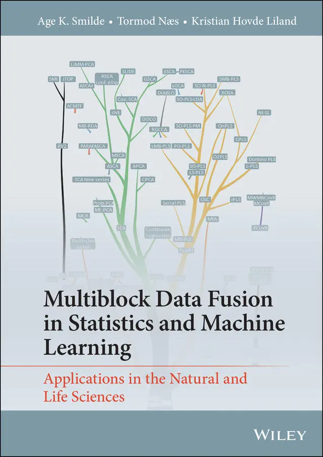
Explore the advantages and shortcomings of various forms of multiblock analysis, and the relationships between them, with this expert guide Multiblock Data Fusion in Statistics and Machine Learning: Applications in the Natural and Life Sciences
Multiblock Data Fusion in Statistics and Machine Learning: Applications in the Natural and Life Sciences
Multiblock Data Fusion in Statistics and Machine Learning — читать онлайн ознакомительный отрывок
Ниже представлен текст книги, разбитый по страницам. Система сохранения места последней прочитанной страницы, позволяет с удобством читать онлайн бесплатно книгу «Multiblock Data Fusion in Statistics and Machine Learning», без необходимости каждый раз заново искать на чём Вы остановились. Поставьте закладку, и сможете в любой момент перейти на страницу, на которой закончили чтение.
Интервал:
Закладка:
1.9 Overview and Links
In this book we will consider a multitude of methods. To streamline this a bit, we are going to give a summary, at the beginning of each chapter, of the methods and aspects which will be discussed. That will be done in the format of a table. We will specify the following aspects of the methods:
1 A method for unsupervised (U), supervised (S) or complex (C) data structures.
2 The method can deal with heterogeneous data (HET, i.e., different measurement scales) or can only deal with homogeneous data (HOM).
3 A method that uses a sequential (SEQ) or simultaneous (SIM) approach.
4 The method is defined in terms of a model (MOD) or in terms of an algorithm (ALG).
5 A method for finding common (C); common and distinct (CD); or finding common, local and distinct components (CLD).
6 Estimation of the model parameters is based on least squares (LS), maximum likelihood (ML), eigenvalue decompositions (ED) or maximising covariance or correlations (MC).
The first item (A) is used to organise the different chapters. Some methods can deal with data of different measurements scales (heterogeneous data) and some methods can only handle homogeneous data. The difference between the simultaneous and sequential method is explained in more detail in Chapter 2. Some methods are defined by a clear model and some methods are based on an algorithm. The already discussed topic of common and distinct variation is also a distinguishing and important feature of the methods and the sections in some of the chapters are organised according to this principle. Finally, there are different ways of estimating the parameters (weights, scores, loadings, etc.) of the multiblock models. This is also explained in more detail in Chapter 2.
Table 1.1is an example of such a table for Chapter 6. This table presents a birds-eye view of the properties of the methods. Each chapter discussing methods will start with this table to set the scene. We will end most chapters with some recommendations for practitioners on what method to use in which situation.
Table 1.1 Overview of methods. Legend: U = unsupervised, S = supervised, C = complex, HOM = homogeneous data, HET = heterogeneous data, SEQ = sequential, SIM = simultaneous, MOD = model-based, ALG = algorithm-based, C = common, CD = common/distinct, CLD = common/local/distinct, LS = least squares, ML = maximum likelihood, ED =eigendecomposition, MC = maximising correlations/covariances. For abbreviations of the methods, see Section 1.11
| A | B | C | D | E | F | ||||||||||||
|---|---|---|---|---|---|---|---|---|---|---|---|---|---|---|---|---|---|
| Section | U | S | C | HOM | HET | SEQ | SIM | MOD | ALG | C | CD | CLD | LS | ML | ED | MC | |
| ASCA | 6.1 | ||||||||||||||||
| ASCA+ | 6.1.3 | ||||||||||||||||
| LiMM-PCA | 6.1.3 | ||||||||||||||||
| MSCA | 6.2 | ||||||||||||||||
| PE-ASCA | 6.3 |
1.10 Notation and Terminology
Throughout this book, we will make use of the following generic notation. When needed, extra notation is explained in local paragraphs. For notational ease, we will not make a distinction between population and estimated weights, scores and loadings which is the tradition in chemometrics and data analysis. For regression equations, when natural we do make that distinction and there we will use the symbol b^ or y^ for the estimated parameters or fitted values.
| x | a scalar |
| x | column vector: bold lowercase |
| X | matrix: bold uppercase |
| Xt | transpose of X |
| X_ | three-way array: bold uppercase underlined |
| m = 1,…, M | index for block |
| im = 1,…, Im | index for first way (e.g., sample) in block m (not shared first way) |
| i = 1,…, I | index for first shared way of blocks |
| jm = 1,…, Jm | index for second way (e.g., variable) in block m (not shared second way) |
| j = 1,…, J | index for second shared way of blocks |
| r = 1,…, R | index for latent variables/principal components |
| R | matrix used to compute scores for PLS |
| Xm | block m |
| xmi | i-th row of Xm (a column vector) |
| xmj | j-th column of Xm (a column vector) |
| W | matrix of weights |
| IL | identity matrix of size L×L |
| T | score matrix |
| P | loading matrix |
| E,F | matrices of residuals |
| 1L | column vector of ones of length L |
| diag(D) | column vector containing the diagonal of D |
| ⊗ | Kronecker product |
| ⊙ | Khatri–Rao product (column-wise Kronecker product) |
| * | Hadamard or element-wise product |
| ⊕ | Direct sum of spaces |
When we discuss methods with only one X- and one Y-block we will use the indices JX and JY for the number of variables in the X- and Y-block, respectively. When there are multiple X-blocks, we will differentiate between the number of variables in the X-blocks using the indices Jm(m=1,…,M); for the Y-block we will then use simply the index J. We try to be as consistent as possible as far as terminology is concerned. Hence, we will use the terms scores, loadings, and weights throughout (see Figure 1.2 and the surrounding text). We will also use the term explained variance which is a slight abuse of the term variance, since it does not pertain to the statistical notion of variance. However, since it is used widely, we will use the term explained variance instead of explained variation as much as possible. Sometimes we need to use a predefined symbol (such as P) in an alternative meaning in order to harmonise the text. We will make this explicit at those places.
1.11 Abbreviations
In this book we will use a lot of abbreviations. Below follows a table with abbreviations used including the chapter(s) in which they appear. A small character ‘s’ in front of an abbreviation means ‘sparse’, e.g., sMB-PLS is the method sparse MB-PLS. For many methods mentioned below there are sparse versions; such as sPCA, sPLS, sSCA, sGCA, sMB-PLS and sMB-RDA. These are not mentioned explicitly in the table.
Table 1.2Abbreviations of the different methods
| Abbreviation | Full Description | Chapter |
|---|---|---|
| ACMTF | Advanced coupled matrix tensor factorisation | 5 |
| ASCA | ANOVA-simultaneous component analysis | 6 |
| BIBFA | Bayesian inter-battery factor analysis | 9 |
| DIABLO | Data integration analysis biomarker latent component omics | 9 |
| DI-PLS | Domain-invariant PLS | 10 |
| DISCO | Distinct and common components | 5 |
| ED-CMTF | Exponential dispersion CMTF | 9 |
| ESCA | Exponential family Simultaneous Component Analysis | 5 |
| GAS | Generalised association study | 4,9 |
| GAC | Generalised association coefficient | 4 |
| GCA | Generalised canonical analysis | 2,5,7 |
| GCD | General coefficient of determination | 4 |
| GCTF | Generalised coupled tensor factorisation | 9 |
| GFA | Group factor analysis | 9 |
| GPA | Generalised Procrustes analysis | 9 |
| GSCA | Generalised simultaneous component analysis | 5 |
| GSVD | Generalised singular value decomposition | 9 |
| IBFA | Inter-battery factor analysis | 9 |
| IDIOMIX | INDORT for mixed variables | 9 |
| INDORT | Individual differences scaling with orthogonal constraints | 9 |
| JIVE | Joint and individual variation explained | 5 |
| LiMM-PCA | Linear mixed model PCA | 6 |
| L-PLS | PLS regression for L-shaped data sets | 8 |
| MB-PLS | Multiblock partial least squares | 7 |
| MB-RDA | Multiblock redundancy analysis | 10 |
| MBMWCovR | Multiblock multiway covariates regression | 10 |
| MCR | Multivariate curve resolution | 5,8 |
| MFA | Multiple factor analysis | 5 |
| MOFA | Multi-omics factor analysis | 9 |
| OS | Optimal-scaling | 2,5 |
| PCA | Principal component analysis | 2,5,8 |
| PCovR | Principal covariates regression | 2 |
| PCR | Principal component regression | 2 |
| PESCA | Penalised ESCA | 9 |
| PE-ASCA | Penalised ASCA | 6 |
| PLS | Partial least squares | 2 |
| PO-PLS | Parallel and orthogonalised PLS regression | 7 |
| RDA | Redundancy analysis | 7 |
| RGCCA | Regularized generalized canonical correlation analysis | 5 |
| RM | Representation matrix approach | 9 |
| ROSA | Response oriented sequential alternation | 7 |
| SCA | Simultaneous component analysis | 2,5 |
| SLIDE | Structural learning and integrative decomposition | 9 |
| SMI | Similarity of matrices index | 4 |
| SO-PLS | Sequential and orthogonalised PLS regression | 7,10 |
Notes
Интервал:
Закладка:
Похожие книги на «Multiblock Data Fusion in Statistics and Machine Learning»
Представляем Вашему вниманию похожие книги на «Multiblock Data Fusion in Statistics and Machine Learning» списком для выбора. Мы отобрали схожую по названию и смыслу литературу в надежде предоставить читателям больше вариантов отыскать новые, интересные, ещё непрочитанные произведения.


Обсуждение, отзывы о книге «Multiblock Data Fusion in Statistics and Machine Learning» и просто собственные мнения читателей. Оставьте ваши комментарии, напишите, что Вы думаете о произведении, его смысле или главных героях. Укажите что конкретно понравилось, а что нет, и почему Вы так считаете.