Stephen J. Mildenhall - Pricing Insurance Risk
Здесь есть возможность читать онлайн «Stephen J. Mildenhall - Pricing Insurance Risk» — ознакомительный отрывок электронной книги совершенно бесплатно, а после прочтения отрывка купить полную версию. В некоторых случаях можно слушать аудио, скачать через торрент в формате fb2 и присутствует краткое содержание. Жанр: unrecognised, на английском языке. Описание произведения, (предисловие) а так же отзывы посетителей доступны на портале библиотеки ЛибКат.

- Название:Pricing Insurance Risk
- Автор:
- Жанр:
- Год:неизвестен
- ISBN:нет данных
- Рейтинг книги:4 / 5. Голосов: 1
-
Избранное:Добавить в избранное
- Отзывы:
-
Ваша оценка:
Pricing Insurance Risk: краткое содержание, описание и аннотация
Предлагаем к чтению аннотацию, описание, краткое содержание или предисловие (зависит от того, что написал сам автор книги «Pricing Insurance Risk»). Если вы не нашли необходимую информацию о книге — напишите в комментариях, мы постараемся отыскать её.
A comprehensive framework for measuring, valuing, and managing risk Pricing Insurance Risk: Theory and Practice
Pricing Insurance Risk: Theory and Practice
Pricing Insurance Risk — читать онлайн ознакомительный отрывок
Ниже представлен текст книги, разбитый по страницам. Система сохранения места последней прочитанной страницы, позволяет с удобством читать онлайн бесплатно книгу «Pricing Insurance Risk», без необходимости каждый раз заново искать на чём Вы остановились. Поставьте закладку, и сможете в любой момент перейти на страницу, на которой закончили чтение.
Интервал:
Закладка:
The Cases share several common characteristics.
Each includes two units, one lower risk and one higher.
Reinsurance is applied to the riskier unit.
Total unlimited losses are calibrated to ¤ 100. (The symbol ¤ denotes a generic currency.)
Losses are in ¤ millions, although the actual unit is irrelevant.
For each Case Study:
Figures 2.2, 2.4, and 2.6 show densities. The horizontal axis shows loss amount. In each figure the top row shows gross losses and the bottom row shows net. The left column uses a linear scale and the right a log scale.
Figures 2.3, 2.5, and 2.7 show bivariate plots of one unit against the other. The three plots show the gross and net logdensities, and the right plot shows a scatter plot of a sample. The two units are assumed independent. These plots show where the bivariate distribution is concentrated.
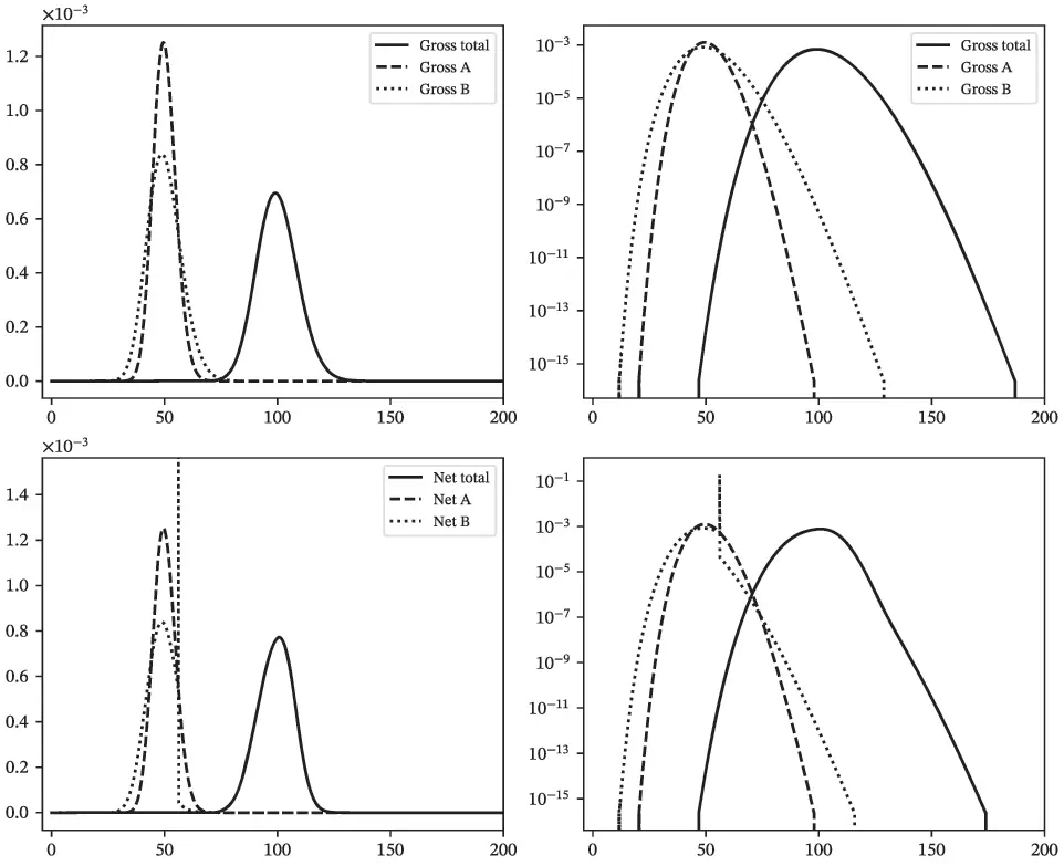
Figure 2.2 Tame Case Study, gross (top) and net (bottom) densities on a nominal (left) and log (right) scale.
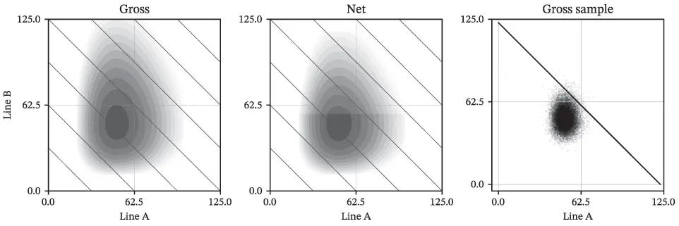
Figure 2.3 Tame Case Study, bivariate densities: gross (left), net (center), and a sample from gross (right). Impact of reinsurance is clear in net plot.
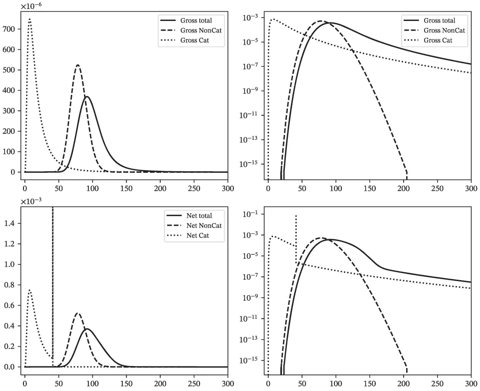
Figure 2.4 Cat/Non-Cat Case Study, gross (top) and net (bottom) densities on a nominal (left) and log (right) scale.
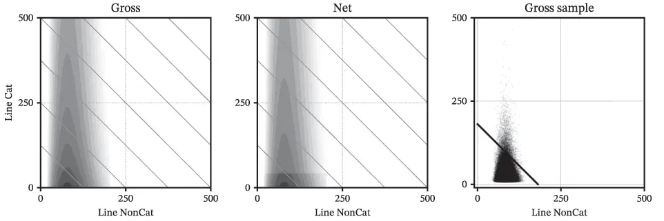
Figure 2.5 Cat/Non-Cat Case Study, bivariate densities: gross (left), net (center), and a sample from gross (right). Impact of reinsurance is clear in net plot.
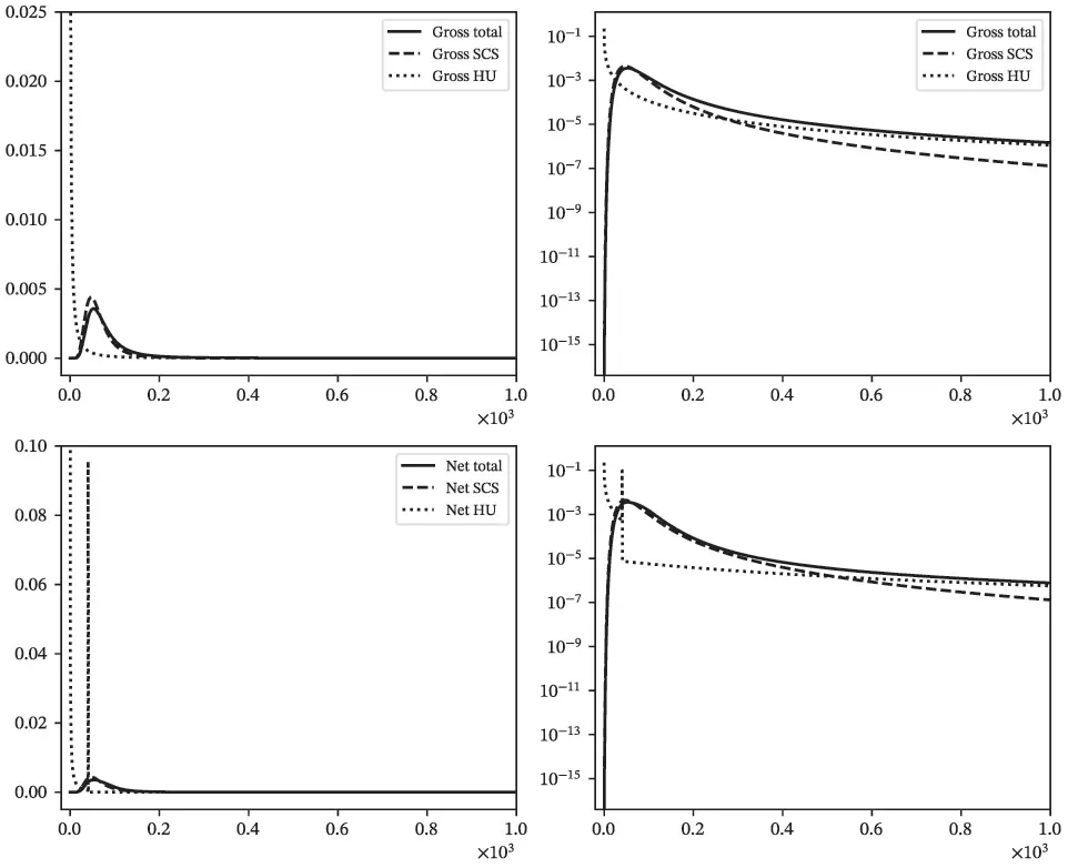
Figure 2.6 Hu/SCS Case Study, gross (top) and net (bottom) densities on a nominal (left) and log (right) scale.
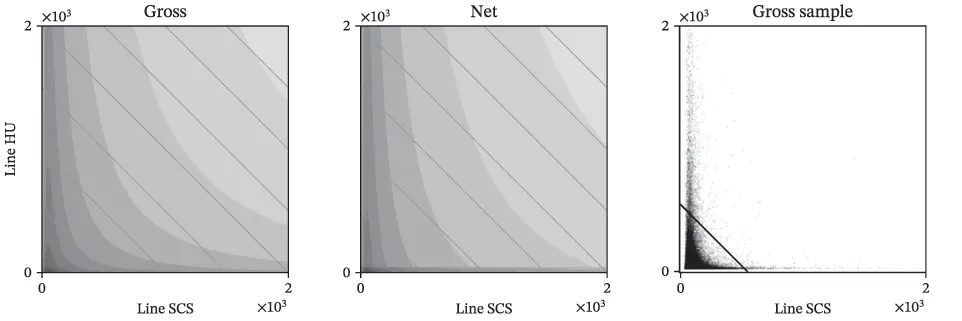
Figure 2.7 Hu/SCS Case Study, bivariate densities: gross (left), net (center), and a sample from gross (right). Impact of reinsurance is clear in net plot.
We strongly recommend that the reader reproduce the Examples and Cases. We suggest a general-purpose programming language such as R or Python, although SQL or even a spreadsheet suffices, with a bit of ingenuity. See Section 2.4.5 for a discussion of the implementation we used.
2.4.1 The Simple Discrete Example
Ins Co. writes two units taking on loss values X1=0, 8, or 10, and X2=0, 1, or 90. The units are independent and sum to the portfolio loss X=X1+X2. The outcome probabilities are 1/2,1/4, and 1/4, respectively, for each marginal. The nine possible outcomes, with associated probabilities, are presented in Table 2.2. The output is typical of that produced by a catastrophe, capital, or pricing simulation model—albeit much simpler.
Exercise 1
Recreate Table 2.2in a spreadsheet (or R or Python). Compute and plot the distribution and survival functions, Pr(X≤x) and Pr(X>x) for X .
Solution.Since the data is discrete, the answers are step functions. The survival function is
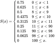 (2.1)
(2.1)
Table 2.2 Simple Discrete Example with nine possible outcomes
| X1 | X2 | X | P(X1) | P(X2) | P(X) |
|---|---|---|---|---|---|
| 0 | 0 | 0 | 1/2 | 1/2 | 1/4 |
| 0 | 1 | 1 | 1/2 | 1/4 | 1/8 |
| 0 | 90 | 90 | 1/2 | 1/4 | 1/8 |
| 8 | 0 | 8 | 1/4 | 1/2 | 1/8 |
| 8 | 1 | 9 | 1/4 | 1/4 | 1/16 |
| 8 | 90 | 98 | 1/4 | 1/4 | 1/16 |
| 10 | 0 | 10 | 1/4 | 1/2 | 1/8 |
| 10 | 1 | 11 | 1/4 | 1/4 | 1/16 |
| 10 | 90 | 100 | 1/4 | 1/4 | 1/16 |
Loss statistics are shown in Table 2.3. The table includes the impact of aggregate reinsurance on the more volatile unit X 2limiting losses to 20 and show a gross and net view for some exhibits. Others are left as Practice questions.
Table 2.3 Discrete Example estimated mean, CV, skewness and kurtosis by line and in total, gross and net. Aggregate reinsurance applied to X2 with an attachment probability 0.25 (¤ 20) and detachment probability 0.0 (¤ 100)
| Gross | Net | |||||
|---|---|---|---|---|---|---|
| Statistic | X1 | X2 | Total | X1 | X2 | Total |
| Mean | 4.500 | 22.750 | 27.250 | 4.500 | 5.250 | 9.750 |
| CV | 1.012 | 1.707 | 1.435 | 1.012 | 1.624 | 0.991 |
| Skewness | 0.071 | 1.154 | 1.131 | 0.071 | 1.147 | 0.794 |
| Kurtosis | −1.905 | −0.667 | −0.649 | −1.905 | −0.673 | −0.501 |
2.4.2 Tame Case Study
In the Tame Case Study, Ins Co. writes two predictable units with no catastrophe exposure. We include it to demonstrate an idealized risk-pool: it represents the best case—from Ins Co.’s perspective. It could proxy a portfolio of personal and commercial auto liability.
To simplify simulations and emphasize the underlying differences between the two units, the Case Study uses a straightforward stochastic model. The two units are independent and have gamma loss distributions with parameters shown in Table 2.4.
Table 2.4 Loss distribution assumptions for each Case Study. The Hu/SCS Case combines a Poisson frequency and lognormal severity
| Case | Unit | Distribution | Mean | CV | Frequency | µ | σ |
|---|---|---|---|---|---|---|---|
| Tame | A | Gamma | 50 | 0.10 | |||
| B | Gamma | 50 | 0.15 | ||||
| Cat/Non-Cat | Non-Cat | Gamma | 80 | 0.15 | |||
| Cat | Lognormal | 20 | 1.0 | 2.649 | 0.833 | ||
| Hu/SCS | Hu | Aggregate | 30 | 10.923 | 2 | −0.417 | 2.5 |
| SCS | Aggregate | 70 | 0.736 | 70 | 1.805 | 1.9 |
The Case includes a gross and net view. Net applies aggregate reinsurance to the more volatile unit B with an attachment probability 0.2 (¤ 56) and detachment probability 0.01 (¤ 69).
Читать дальшеИнтервал:
Закладка:
Похожие книги на «Pricing Insurance Risk»
Представляем Вашему вниманию похожие книги на «Pricing Insurance Risk» списком для выбора. Мы отобрали схожую по названию и смыслу литературу в надежде предоставить читателям больше вариантов отыскать новые, интересные, ещё непрочитанные произведения.


Обсуждение, отзывы о книге «Pricing Insurance Risk» и просто собственные мнения читателей. Оставьте ваши комментарии, напишите, что Вы думаете о произведении, его смысле или главных героях. Укажите что конкретно понравилось, а что нет, и почему Вы так считаете.