Mohamed-Aymen Chalouf - Intelligent Security Management and Control in the IoT

[2.4]

The modeled system is an approximation of reality in many ways, especially where it concerns the fixed and limited number of access attempts. However, we preferred to simplify the model to make it more tractable (Figure 2.5).

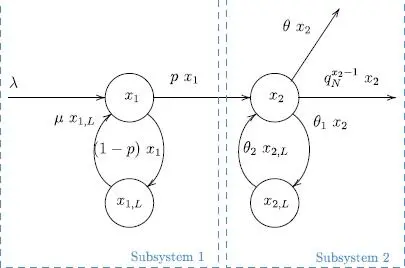
Figure 2.5. System model. For a color version of this figure, see www.iste.co.uk/chalouf/intelligent.zip

The sub-system 1 represents the terminals that wish to connect; the IoT devices belonging to the state variable x 1represent those that can try to connect with a probability p ; in case of failure, they go into the waiting state x 1,Lfor a set duration. Sub-system 2 represents the IoT devices that can try to choose a preamble. In case of collision, they can try to access it several times. Each quits sub-system 2 when it succeeds in being the only one to have chosen a preamble or when it reaches the maximum number of attempts (with a rate of θ ).

The proposed model is fluid: the quantities involved and the whole numbers are considered to be real (continuous) quantities. The parameters used are listed below:

– x1(t) is the number of waiting devices;

– x1,L(t) is the number of blocked devices, after a failure at the end of an access attempt (i.e. ACB);

– x2(t) is the total number of devices that pass the ACB control and wait to start the random access attempt (RA);

– x2,L(t) is the number of blocked devices, at instant t, after a failed RA attempt, awaiting a new attempt;

– λ is the arrival rate of IoT objects;

– μ is the rate of objects that can reattempt ACB after a failure;

– θ1 is the RA failure rate, which is equal to when θ is equal to 0 (see the point before last);

– θ2 is the rate of objects that can attempt access after a failure;

– θ is the rate at which the device abandons transmission after having reached the maximum number of RA attempts; in a correctly dimensioned system, we should have θ = 0;

– p is the ACB blocking factor.

We are now able to describe the evolution of state variables 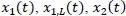and basing our study on the model represented in Figure 2.5. The model’s dynamic is described by the following system of differential equations:

[2.5]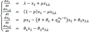

In what follows, we suppose that θ = 0, to simplify the model. In fact, a system where the devices often reach the maximum number of attempts is an unstable system, which we naturally try to avoid.

The model described in [2.5] is nonlinear and not affine, in the control. It can easily be demonstrated that the model described is not observable, in view of its state [ x 1 x 1,L x 2 x 2,L ]which cannot be known precisely. It is also not controllable, as the blocking factor p can only act partially on the state. These properties render the synthesis of an optimal controller, guaranteeing the stability of the very complex system, described above, very complex.

Although the state is not observable, it is possible to produce an estimation of the average number of devices attempting access by reversing equations [2.1]and [ 2.3]. This gives a very noisy measurement, but one which is, nevertheless, useful for IoT blocking as we demonstrated in Bouzouita et al. (2019).

The difficulty of observing the system state, described in section 2.4, has led us to consider strategies making it possible to deduce the blocking factor even in the presence of very noisy measurements.

It is in this sense that we relied on deep learning techniques, which demonstrated great effectiveness in automatically extracting characteristics of system “features” in the presence of data tainted with noise or even of incomplete data (Rolnick et al. 2017).

Given the lack of data, we have considered the class of reinforcement learning techniques.

More particularly, we considered the “Twin Delayed Deep Deterministic policy gradient algorithm” (TD3) technique, which can tackle a continuous action space, and which has shown greater effectiveness in learning speed and in performance than existing approaches (Fujimoto et al. 2018).

We formulate, in what follows, the problem of access in the IoT as a reinforcement learning problem, in which an agent finds iteratively a sub-optimal blocking factor, making it possible to reduce the access conflict.

In reinforcement learning (Sutton et al. 2019), we have two main entities, an environment and an agent. The learning process happens through interaction between these entities so that the agent can optimize a total revenue. At each stage t , the agent obtains a representation of the state St of the environment and chooses an action at , based on this. Then the agent applies this action to the environment. Consequently, the environment passes to a new state S t+1and the agent receives a recompense rt . This interaction can be modeled as a Markovian decision process (MDP) M = (S, A, P, R) , where S is the state space, A the action space, P the dynamic transition and R the revenue function. The behavior of the agent is defined by its policy π: S ⟶ A , which makes it possible to link a state to an action where a deterministic system is involved, or a distribution of action where it is probabilistic. The objective of such a system is to find the optimal policy π* , making it possible to maximize the accumulated revenue.

In the problem of controlling access to the IoT, we define a discrete MDP, where the state, the action and the revenue are defined as follows:

– The state: given that the number of terminals attempting access at a given instant k is unavailable, the state we are considering is based on measured estimates. Since a single measurement of this number is necessarily very noisy, we will consider a set of several measurements, which can better reveal the state present in the network. The state sk is defined as the vector , where H represents the measurement horizon.

– The action: at each state, the agent must select the blocking factor p which will need to be considered by the IoT objects. This value is continuous and determinist in the problem that we consider, that is that the same state sk will always give the same action ak.

– The revenue: this is a signal that the agent receives from the environment after the execution of an action. Thus, at stage k, the agent obtains a revenue rk as a consequence of the action ak that it carried out in state sk. This revenue will allow the agent to know the quality of the action executed, the objective of the agent being to maximize this revenue.