Kip Thorne - The Science of Interstellar

My code was very slow and had low resolution. Oliver’s challenge was to convert my equations into computer code that could generate the ultra-high-quality IMAX images needed for the movie.

Oliver and I did this in steps. We began with a nonspinning black hole and a nonmoving camera. Then we added the black hole’s spin. Then we added the camera’s motion: first motion in a circular orbit, and then plunging into a black hole. And then we switched to a camera around a wormhole.

At this point, Oliver hit me with a minibombshell: To model some of the more subtle effects, he would need not only equations describing the trajectory of a ray of light, but also equations describing how the cross section of a beam of light changes its size and shape during its journey past the black hole.

I knew more or less how to do this, but the equations were horrendously complicated and I feared making mistakes. So I searched the technical literature and found that in 1977 Serge Pineault and Rob Roeder at the University of Toronto had derived the necessary equations in almost the form I needed. After a three-week struggle with my own stupidities, I brought their equations into precisely the needed form, implemented them in Mathematica, and wrote them up for Oliver, who incorporated them into his own computer code. At last his code could produce the quality images needed for the movie.

At Double Negative, Oliver’s computer code was just the beginning. He handed it over to an artistic team led by Eugénie von Tunzelmann, who added an accretion disk (Chapter 9) and created the background galaxy with its stars and nebulae that Gargantua would lens. Her team then added the Endurance and Rangers and landers and the camera animation (its changing motion, direction, field of view, etc.), and molded the images into intensely compelling forms: the fabulous scenes that actually appear in the movie. For further discussion, see Chapter 9.

In the meantime, I puzzled over the high-resolution film clips that Oliver and Eugénie sent me, struggling to extract insights into why the images look like they look, and why the star fields stream as they stream. For me, those film clips are like experimental data: they reveal things I never could have figured out on my own, without those simulations—for example, the things I described in the previous section (Figures 8.5 and 8.6). We plan to publish one or more technical papers, describing the new things we learned.

Although Chris chose not to show any gravitational slingshots in Interstellar , I wondered what they would look like to Cooper as he piloted the Ranger toward Miller’s planet. So I used my equations and Mathematica to simulate them and produce images. (My images have far lower resolution than Oliver’s and Eugénie’s due to my code’s slowness.)

Figure 8.7 shows a sequence of images, as Cooper’s Ranger swings around an intermediate-mass black hole (IMBH) to initiate its descent toward Miller’s planet—in my scientist’s interpretation of Interstellar . This is the slingshot described in Figure 7.2.

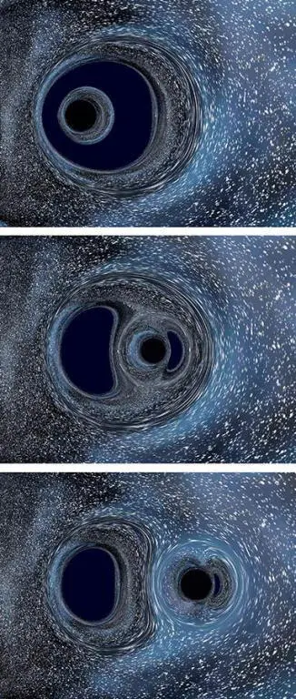
In the top image, Gargantua is in the background with the IMBH passing in front of it. The IMBH grabs light rays from distant stars that are headed toward Gargantua, swings the rays around itself, and ejects them toward the camera. This explains the donut of starlight that surrounds the IMBH’s shadow. Although the IMBH is a thousand times smaller than Gargantua, it is far closer to the Ranger than is Gargantua, so it looks only modestly smaller.

As the IMBH appears to move rightward, as seen by the slingshot-moving camera, it leaves Gargantua’s primary shadow behind itself (middle picture in Figure 8.7), and it pushes a secondary image of Gargantua’s shadow ahead of itself. These two images are completely analogous to the primary and secondary images of a star gravitationally lensed by a black hole; but now it is Gargantua’s shadow that is being lensed, by the IMBH. In the bottom picture, the secondary shadow is shrinking in size, as the IMBH moves onward. By this time the slingshot is nearly complete, and the camera, on board the Ranger, is headed downward, toward Miller’s planet.

As impressive as these images may be, they can be seen only up close to the IMBH and Gargantua, not from the great distance of Earth. To astronomers on Earth, the most visually impressive things about gigantic black holes are jets that stick out of them and the light from brilliant disks of hot gas that orbit them. To these we’ll now turn.

Most of the objects seen by radio telescopes are huge clouds of gas, clouds far larger than any star. But in the early 1960s a few tiny objects were found. Astronomers named these objects quasars for “quasi-stellar radio sources.”

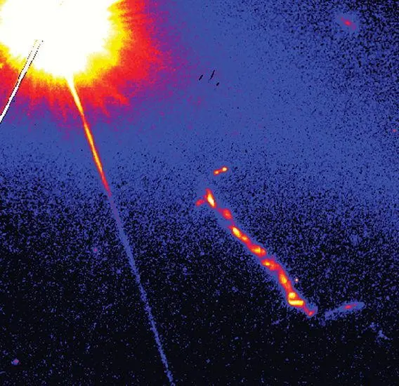
In 1962 the Caltech astronomer Maarten Schmidt, looking through the world’s largest optical telescope on Palomar Mountain, discovered light coming from a quasar called 3C273. It looked like a bright star with a faint jet shooting out of it (Figure 9.1). This was weird!

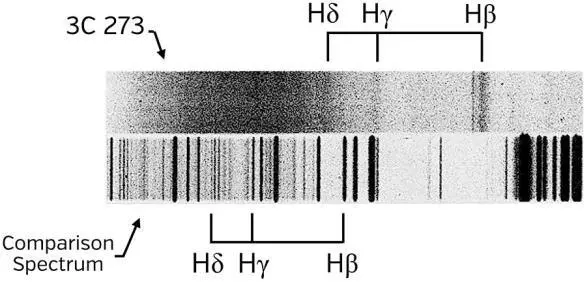
When Schmidt split 3C273’s light into its various colors (as is sometimes done by sending light through a prism), he saw the set of spectral lines in the bottom of Figure 9.1. At first sight, these were unlike any spectral lines he had ever seen. But in February 1963, after a few months’ struggle, he realized the lines were unfamiliar simply because their wavelengths were 16 percent larger than normal. This is called the Doppler shift; it was caused by the quasar’s moving away from Earth at 16 percent the speed of light, about c /6. What could cause that ultrafast motion? The least crazy explanation Schmidt could find was the expansion of the universe.

As the universe expands, objects far from Earth move apart from us at very high speed, and objects nearer move away more slowly. 3C273’s enormous speed, one-sixth that of light, meant that 3C273 was 2 billion light-years from Earth, nearly the farthest object that had ever been seen at that time. From its brightness and its distance, Schmidt concluded that 3C273 puts out 4 trillion times more power in light than the Sun, and a hundred times more power than the brightest galaxies!

This prodigious power fluctuated on times as short as a month, so most of the light must be coming from an object so small that the light can travel across it in one month’s time—far smaller than the distance from Earth to the nearest star, Proxima Centauri. And other quasars with almost as much power fluctuated on times of a few hours, so they had to be not much larger than our solar system. One hundred times the power of a bright galaxy, coming from a region the size of our solar system; that was phenomenal!