Andrew Tanenbaum - Distributed operating systems

Computer systems can fail due to a fault in some component, such as a processor, memory, I/O device, cable, or software. A faultis a malfunction, possibly caused by a design error, a manufacturing error, a programming error, physical damage, deterioration in the course of time, harsh environmental conditions (it snowed on the computer), unexpected inputs, operator error, rodents eating part of it, and many other causes. Not all faults lead (immediately) to system failures, but some do.

Faults are generally classified as transient, intermittent, or permanent. Transient faultsoccur once and then disappear. if the operation is repeated, the fault goes away. A bird flying through the beam of a microwave transmitter may cause lost bits on some network (not to mention a roasted bird). If the transmission times out and is retried, it will probably work the second time.

An intermittent faultoccurs, then vanishes of its own accord, then reappears, and so on. A loose contact on a connector will often cause an intermittent fault. Intermittent faults cause a great deal of aggravation because they are difficult to diagnose. Typically, whenever the fault doctor shows up, the system works perfectly.

A permanent faultis one that continues to exist until the faulty component is repaired. Burnt-out chips, software bugs, and disk head crashes often cause permanent faults.

The goal of designing and building fault-tolerant systems is to ensure that the system as a whole continues to function correctly, even in the presence of faults. This aim is quite different from simply engineering the individual components to be highly reliable, but allowing (even expecting) the system to fail if one of the components does so.

Faults and failures can occur at all levels: transistors, chips, boards, processors, operating systems, user programs, and so on. Traditional work in the area of fault tolerance has been concerned mostly with the statistical analysis of electronic component faults. Very briefly, if some component has a probability p of malfunctioning in a given second of time, the probability of it not failing for k consecutive seconds and then failing is p(1 – p) k. The expected time to failure is then given by the formula

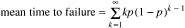
Using the well-known equation for an infinite sum starting at k -1: Σα k=α/(1–α), substituting α=1 –p, differentiating both sides of the resulting equation with respect to p, and multiplying through by – p we see that

For example, if the probably of a crash is 10 -6per second, the mean time to failure is 10 6sec or about 11.6 days.

In a critical distributed system, often we are interested in making the system be able to survive component (in particular, processor) faults, rather than just making these unlikely. System reliability is especially important in a distributed system due to the large number of components present, hence the greater chance of one of them being faulty.

For the rest of this section, we will discuss processor faults or crashes, but this should be understood to mean equally well process faults or crashes (e.g., due to software bugs). Two types of processor faults can be distinguished:

1. Fail-silent faults.

2. Byzantine faults.

With fail-silent faults,a faulty processor just stops and does not respond to subsequent input or produce further output, except perhaps to announce that it is no longer functioning. These are also called fail-stop faults.With Byzantine faults,a faulty processor continues to run, issuing wrong answers to questions, and possibly working together maliciously with other faulty processors to give the impression that they are all working correctly when they are not. Undetected software bugs often exhibit Byzantine faults. Clearly, dealing with Byzantine faults is going to be much more difficult than dealing with fail-silent ones.

The term "Byzantine" refers to the Byzantine Empire, a time (330-1453) and place (the Balkans and modern Turkey) in which endless conspiracies, intrigue, and untruthfulness were alleged to be common in ruling circles. Byzantine faults were first analyzed by Pease et al. (1980) and Lamport et al. (1982). Some researchers also consider combinations of these faults with communication line faults, but since standard protocols can recover from line errors in predictable ways, we will examine only processor faults.

As we have just seen, component faults can be transient, intermittent, or permanent, and system failures can be fail-silent or Byzantine. A third orthogonal axis deals with performance in a certain abstract sense. Suppose that we have a system in which if one processor sends a message to another, it is guaranteed to get a reply within a time T known in advance. Failure to get a reply means that the receiving system has crashed. The time T includes sufficient time to deal with lost messages (by sending them up to n times).

In the context of research on fault tolerance, a system that has the property of always responding to a message within a known finite bound if it is working is said to be synchronous.A system not having this property is said to be asynchronous.While this terminology is unfortunately, since it conflicts with more traditional uses of the terms, it is widely used among workers in fault tolerance.

It should be intuitively clear that asynchronous systems are going to be harder to deal with than synchronous ones. If a processor can send a message and know that the absence of a reply within T sec means that the intended recipient has failed, it can take corrective action. If there is no upper limit to how long the response might take, even determining whether there has been a failure is going to be a problem.

The general approach to fault tolerance is to use redundancy. Three kinds are possible: information redundancy, time redundancy, and physical redundancy. With information redundancy, extra bits are added to allow recovery from garbled bits. For example, a Hamming code can be added to transmitted data to recover from noise on the transmission line.

With time redundancy, an action is performed, and then, if need be, it is performed again. Using the atomic transactions described in Chap. 3 is an example of this approach. If a transaction aborts, it can be redone with no harm. Time redundancy is especially helpful when the faults are transient or intermittent.

With physical redundancy, extra equipment is added to make it possible for the system as a whole to tolerate the loss or malfunctioning of some components. For example, extra processors can be added to the system so that if a few of them crash, the system can still function correctly.

There are two ways to organize these extra processors: active replication and primary backup. Consider the case of a server. When active replication is used, all the processors are used all the time as servers (in parallel) in order to hide faults completely. In contrast, the primary backup scheme just uses one processor as a server, replacing it with a backup if it fails.

We will discuss these two strategies below. For both of them, the issues are:

1. The degree of replication required.

2. The average and worst-case performance in the absence of faults.