Petros Katsafados - Numerical Weather Prediction and Data Assimilation

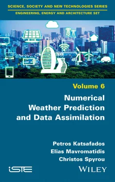
1 Cover

2 Preface

3 Introduction

4 1 The Primitive Equations 1.1. Wind forecast equations (conservation of momentum) 1.2. Continuity equation (conservation of mass) 1.3. Temperature forecast equation (conservation of energy) 1.4. Moisture forecast equation (conservation of water vapor) 1.5. Synopsis of equations

5 2 Solving Methods in NWP Models 2.1. Decomposition of variables – the perturbation method 2.2. Numerical solutions of partial differential equations 2.3. Time splitting

6 3 Domain Structures and Boundary Conditions 3.1. Horizontal grid structure and resolution 3.2. The vertical coordinate system 3.3. Boundary conditions 3.4. Design of a simulation

7 4 Introduction to Data Assimilation 4.1. Successive correction methods 4.2. Least square method 4.3. Variational approach 4.4. Generalization of the methods

8 5 Desert Dust Modeling 5.1. Dust uptake mechanisms formulation 5.2. Dust advection and deposition 5.3. Parameterization of the dust feedbacks on climate

9 6 Simulations of Extreme Weather and Dust Events 6.1. Case study 1: numerical simulation of a Mediterranean cyclone and its sensitivity on lower boundary conditions 6.2. Case study 2: nowcasting an extreme precipitation event 6.3. Case study 3: seasonal predictability of a large-scale heat wave 6.4. Numerical study of a severe desert dust storm over Crete

10 Appendices Appendix 1 Appendix 2

11 References

12 Index

13 End User License Agreement

1 Chapter 1 Table 1.1. Formulae of acceleration due to stress in all directions Table 1.2. Formulae of stresses in all directions Table 1.3. Formulae of resultant acceleration due to stress in all directions

2 Chapter 5Table 5.1. Trimodal size distribution of sources (source: DʼAlmeida 1987; Zender...Table 5.2. Complex refractive index for several atmospheric elements at waveleng...

3 Chapter 6Table 6.1. List of the simulations and their SST characteristicsTable 6.2. Cyclone central MSLP (hPa) as estimated in the numerical simulations....Table 6.3. List of LAPS simulations characteristics including background fields ...Table 6.4. Records of near-surface maximum temperatures at four meteorological s...

1 Chapter 1 Figure 1.1. The direction of centripetal acceleration. The distance between the ... Figure 1.2. A schematic representation of the pressure gradient force (x-compone... Figure 1.3. Two spherical masses (the Earth and an atmospheric element) whose ce... Figure 1.4. Vertical profile of the fluid flow between the fixed lower plate and... Figure 1.5. A differential volume element of fluid with sides declared with δx, ... Figure 1.6. Schematic representation of the relation between the true and the mo... Figure 1.7. Variation of the Coriolis force (ms –2) in accordance with the latitu... Figure 1.8. The influence of a counterclockwise rotating sphere (Earth) to the r... Figure 1.9. Schematic representation of a fixed differential volume element and ... Figure 1.10. A schematic representation of a box of gas as it changes in size, d...

2 Chapter 2Figure 2.1. Finite difference approximations at a point on a continuous functionFigure 2.2. The discretized domainFigure 2.3. Schematic representation of a rectangular grid on two horizontal dim...

3 Chapter 3Figure 3.1. Example of unstaggered grid (top) and staggered grid (bottom), in th...Figure 3.2. Various types of rectangular grids (two horizontal dimensions) accor...Figure 3.3. Schematic representation of coordinate surfaces for (a) z-coordinate...Figure 3.4. Schematic representation of the Eta coordinate systemFigure 3.5. Schematic representation of σ-coordinate surfaces, as defined by equ...

4 Chapter 4Figure 4.1. Schematic of the current global atmospheric observing system. For a ...Figure 4.2. Schematic representation of an NWP model grid structure (dots) with ...Figure 4.3. Illustration of the cost function minimization in a two-variable mod...Figure 4.4. Representation of the operational LAPS domain. For a color version o...

5 Chapter 5Figure 5.1. Schematic plot showing all the physical mechanisms associated with d...Figure 5.2. Processes that initiate desert dust production (source: Shao et al. ...Figure 5.3. Clay content (in %) derived from the global FAO dataset. For a color...Figure 5.4. Specification of the desert fraction. The bold-line and the dashed-l...Figure 5.5. Dust source strength as defined by the August 1–16, 2016 mean NDVI (...Figure 5.6. Boundary layer vertical structure. The red line denotes the change o...Figure 5.7. Settling velocity of dust, as a function of the particle size (sourc...Figure 5.8. Patterns of Rayleigh, Mie and geometric scattering (source: Alkholid...Figure 5.9. Dust radiative feedback in spring in the incoming shortwave (a) and ...Figure 5.10. Total condensates mixing ratio (g kg –1) for the pristine (left colu...

6 Chapter 6Figure 6.1. ECMWF analyses of (a) MSLP (hPa) and (b) absolute vorticity (s −1, in...Figure 6.2. Horizontal distribution of ECMWF SST analysis (°C) valid for January...Figure 6.3. Comparative horizontal plots of the differences (in °C) between (a) ...Figure 6.4. Comparisons of the MSLP (at 4 hPa intervals) for the entire simulati...Figure 6.5. Simulated cyclone trajectories, valid from January 21, 2004, at 18:0...Figure 6.6. Differences of 12-hourly accumulated precipitation (mm), as simulate...Figure 6.7. (a) Geopotential height (solid black lines in gpdam) and MSLP (solid...Figure 6.8. Hourly accumulated precipitation (color shaded in mm) and MSLP (soli...Figure 6.9. Timeplots of the measured accumulated precipitation (histograms in m...Figure 6.10. (a) CTRL00MPE simulation analysis of hourly accumulated precipitati...Figure 6.11. Geopotential height at 500 hPa (solid lines in gpm) and temperature...Figure 6.12. Mean temperature anomalies (°C) for July 2010 with respect to the 1...Figure 6.13. The ensemble structureFigure 6.14. Mean monthly temperature anomaly (K) at 850 hPa for (a) July and (b...Figure 6.15. Spaghetti diagrams (red solid lines) of the mean monthly temperatur...Figure 6.16. Desert dust identification from the MSG-SEVIRI dust RGB images on t...Figure 6.17. Surface analysis chart for March 21, 2018, at 18:00 UTC (source: UK...Figure 6.18. a) WRF-ARW domain configuration, where the three nests are shown. T...Figure 6.19. Spatial distribution of WRF-ARW for a) sand fraction percentage and...Figure 6.20. Mean sea level pressure valid on March 22, 2018, 00:00 UTC, as simu...Figure 6.21. a) Wind speed (in ms −1) at 850 hPa, as simulated by the WRF-ARW mod...Figure 6.22. a) Wind speed at 10 m (in ms −1) and b) surface dust concentration (...

7 AppendixFigure A1.1. Relation between the absolute and the relative velocity at the rota...Figure A1.2. a) Symbols of the spherical coordinate system. R is the radius of t...Figure A2.1. Schematic representation of the relationship between the derivative...

1 Cover

2 Table of Contents

3 Begin Reading

1 v

2 iii

3 iv

4 vii

5 viii

6 ix

7 x

8 1

9 2

10 3

11 4

12 5

13 6

14 7

15 8

16 9

17 10

18 11

19 12

20 13

21 14

22 15

23 16

24 17

25 18

26 19

27 20

28 21