Franco Taroni - Statistics and the Evaluation of Evidence for Forensic Scientists

Apart from their DNA profile, what else is known about the criminal? In particular, is there any information, such as ethnicity, which may be related to their DNA profile? What is the population from which the criminal may be thought to have come? Could they be another member of the family of the PoI?

Questions such as these and their effect on the interpretation and evaluation of evidence will be discussed in greater detail. First, consider only the evidence of the DNA profile in isolation and one particular locus, LDLR . It is no longer used in forensic genetics; it is used here for ease of explanation. Assume the crime was committed in Chicago and that there is eyewitness evidence that the criminal was a Caucasian. Information is available to the investigating officer about the genotypic distribution for the LDLR locus in Caucasians in Chicago and is given in Table 1.1. The information about the location of the crime and the ethnicity of the criminal is relevant. Genotypic population proportions vary across locations and amongst ethnic groups. A PoI is arrested and a swab is taken for a comparative genetic test. For locus LDLR the genotype of the crime stain and that of the PoI correspond. The investigating officer knows a little about probability and works out that the probability of two people chosen at random and unrelated to the suspect having corresponding alleles, using the figures in Table 1.1as estimates of population proportions, is

(1.1)

(see Section 3.5.1). They are not too sure what this result means. Is it high and is a high value incriminating for the PoI? Is it low and is a low value incriminating? In fact, a low value is more incriminating than a high value.

Table 1.1Genotypic relative frequencies for locus LDLR amongst Caucasians in Chicago based on a sample of size 200.

Source: From Johnson and Peterson (1999). Reprinted with permissions of ASTM International.

Genotype
Relative frequency (%)	18.8	32.1	49.1

They think a little more and remembers that, not only do the genotypes correspond, but also that they are both of type . The proportions of genotypes and are not relevant. He works out the probability that two people chosen at random both have genotype as

(see Section 3.5). He is still not too sure what this means but feels that it is more representative of the information available to him than the previous probability, since it takes account of the actual genotypes of the crime stain and the PoI.

The genotype of the crime stain for locus LDLR is . The genotype of the PoI is also (if it were not they would not be a PoI). What is the value of this evidence? The discussion earlier suggests various possible answers.

1 (1) The probability that two people chosen at random have the same genotype for locus LDLR. This is 0.379.

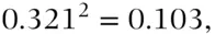
2 (2) The probability that two people chosen at random have the same, pre‐specified, genotype. For genotype this is 0.103.

3 (3) The probability that one person, chosen at random, has the same genotype as the crime stain. If the crime stain is of group , this probability is 0.321, from Table 1.1.

The relative merits of these answers will be discussed in Section 3.5 for (1) and (2) and Section 2.4.5for (3).

The phrase at random is taken to include the caveat that the people chosen are unrelated to the PoI. In practice, the phrase at random is not considered in its scientific usage (a person chosen accordingly to a randomising device). Note that, as expressed by Balding and Steele (2015),

It is important to keep in mind that in any crime investigation, random man is pure fiction: nobody was actually chosen at random in any population, and so probabilities calculated under an assumption of randomly sampled suspects have no direct bearing on evidential weight in actual cases. (p. 160)

A comment on randomness is also made by Kingston and Kirk (1964) (see pp. 515–516). A discussion about the extension of the concept of ‘random man’ to the one of ‘unrelated person’ to the PoI, when dealing with DNA evidence evaluation, is discussed in Milot et al. (2020).

Section 1.3.2discussed an example of the interpretation of the evidence of DNA profiling. Consider now an example concerning glass fragments and the measurement of the refractive index of these.

Example 1.2As before, consider the investigation of a crime. A window has been broken during the commission of the crime. A PoI is found with fragments of glass on their clothing, similar in refractive index to the broken window. Several fragments are taken for investigation and their refractive index measurements taken.

Note that there is a difference here from Example 1.1, where it was assumed that the crime stain had come from the criminal and been transferred to the crime scene. In Example 1.2 glass is transferred from the crime scene to the criminal. Glass on the PoI need not have come from the scene of the crime; it may have come from elsewhere and by perfectly innocent means. This is an asymmetry associated with this kind of scenario. The evidence is known as transfer evidence , as discussed in Section 1.1, because evidence (e.g. blood or glass fragments) has been transferred from the criminal to the scene or vice versa . Transfer from the criminal to the scene has to be considered differently from evidence transferred from the scene to the criminal. A full discussion of this is given in Chapters 5and 6.

Comparison in Example 1.2 has to be made between the two sets of fragments on the basis of their refractive index measurements. The evidential value of the outcome of this comparison has to be assessed. Notice that it is assumed that none of the fragments has any distinctive features and comparison is based only on the refractive index measurements.

Methods for evaluating such evidence were discussed in many papers in the late 1970s and early 1980s Evett (1977, 1978), Evett and Lambert (1982, 1984, 1985), Grove (1981, 1984), Lindley (1977c), Seheult (1978), and Shafer (1982). These methods will be described as appropriate in Chapters 3 and 7. Knowledge‐based computer systems have been developed. See Curran and Hicks (2009) and Curran (2009) for a review of practices in the forensic evaluation of glass and DNA evidence. As an aside, sophisticated systems have been developed to deal with DNA, notably DNA mixtures complexities (i.e. number of donors, peaks heights). Examples are presented and evaluated in Bright et al. (2016), Alladio et al. (2018), and Bleka et al. (2019).