Malcolm L. Hunter - Fundamentals of Conservation Biology
Здесь есть возможность читать онлайн «Malcolm L. Hunter - Fundamentals of Conservation Biology» — ознакомительный отрывок электронной книги совершенно бесплатно, а после прочтения отрывка купить полную версию. В некоторых случаях можно слушать аудио, скачать через торрент в формате fb2 и присутствует краткое содержание. Жанр: unrecognised, на английском языке. Описание произведения, (предисловие) а так же отзывы посетителей доступны на портале библиотеки ЛибКат.
- Название:Fundamentals of Conservation Biology
- Автор:
- Жанр:
- Год:неизвестен
- ISBN:нет данных
- Рейтинг книги:3 / 5. Голосов: 1
-
Избранное:Добавить в избранное
- Отзывы:
-
Ваша оценка:
Fundamentals of Conservation Biology: краткое содержание, описание и аннотация
Предлагаем к чтению аннотацию, описание, краткое содержание или предисловие (зависит от того, что написал сам автор книги «Fundamentals of Conservation Biology»). Если вы не нашли необходимую информацию о книге — напишите в комментариях, мы постараемся отыскать её.
has been a valued mainstay of the literature, serving both to introduce new students to this ever-changing topic, and to provide an essential resource for academics and researchers working in the discipline. In the decade since the publication of the third edition, concerns about humanity’s efforts to conserve the natural world have only grown deeper, as new threats to biodiversity continue to emerge.
This fourth edition has taken into account a vast new literature, and boasts nearly a thousand new references as a result. By embracing new theory and practice and documenting many examples of both conservation successes and the hard lessons of real-world “wicked” environmental problems,
remains a vital resource for biologists, conservationists, ecologists, environmentalists, and others.
Fundamentals of Conservation Biology — читать онлайн ознакомительный отрывок
Ниже представлен текст книги, разбитый по страницам. Система сохранения места последней прочитанной страницы, позволяет с удобством читать онлайн бесплатно книгу «Fundamentals of Conservation Biology», без необходимости каждый раз заново искать на чём Вы остановились. Поставьте закладку, и сможете в любой момент перейти на страницу, на которой закончили чтение.
Интервал:
Закладка:
Table 5.3 The proportion of genetic variation retained in small populations of constant size after 1, 5, 10, and 100 generations is approximately [1 − 1/(2 N )] t, where N is the population size and t is the number of generations. For example, 0.95 5= 0.77.
Based on Frankel and Soulé 1981
| Generations | ||||
|---|---|---|---|---|
| Population size (N) | 1 | 5 | 10 | 100 |
| 2 | 0.75 | 0.24 | 0.06 | <<0.01 |
| 6 | 0.917 | 0.65 | 0.42 | <<0.01 |
| 10 | 0.95 | 0.77 | 0.60 | <0.01 |
| 20 | 0.975 | 0.88 | 0.78 | 0.08 |
| 50 | 0.99 | 0.95 | 0.90 | 0.36 |
| 100 | 0.995 | 0.975 | 0.95 | 0.60 |
We can see that although a population of 10 individuals may retain 95% of its genetic variation after one generation (or after one bottleneck), with random genetic drift for 10 generations only 60% of the variation is likely to be retained, and after 100 generations virtually all the original genetic variation would be lost. A similar pattern exists for the loss of alleles; after many generations of random genetic drift, small populations will usually retain only one allele for a given gene ( Table 5.4). In the language of genetics, the gene will have been fixed for that allele. In sum, random genetic drift in a population that remains small for many generations is much more likely to lead to a loss of genetic diversity than is a single bottleneck from which a population recovers quickly.
Table 5.4 Expected number of alleles remaining after t generations for a population of six individuals with 2, 4, or 12 alleles for a gene, assuming equal frequency of each allele.
Based on Frankel and Soulé 1981
| Number of alleles | |||
|---|---|---|---|
| Generations | m = 2 | m = 4 | m = 12 |
| 0 | 2.00 | 4.00 | 12.00 |
| 1 | 1.99 | 3.87 | 7.78 |
| 2 | 1.99 | 3.55 | 5.88 |
| 8 | 1.67 | 2.18 | 2.64 |
| 20 | 1.24 | 1.36 | 1.44 |
| ∞ | 1.00 | 1.00 | 1.00 |
If drift erodes genetic diversity then will mutation simply replenish it? Probably not. The problem is a severe imbalance between the rates at which the two processes operate. A population bottleneck can deplete genetic diversity from a population during just a few generations if the bottleneck is narrow enough. In contrast, it has been estimated that 10 5–10 7generations are required to regenerate allelic diversity for a single gene (Lande and Barrowclough 1987). The genetic machinery of a cell is remarkable at avoiding “copying errors” and thus we cannot rely on mutation to replenish genetic diversity over time scales of conservation concern; preventing bottlenecks and excessive genetic drift by keeping populations of “healthy” size is our best approach.
Effective Population Size
To estimate the effects of bottlenecks and random genetic drift, as presented in Tables 5.2and 5.3, we made some simplifying assumptions: that the organism is diploid, sexually reproducing, and has nonoverlapping generations; that the population is of constant size, has equal numbers of females and males, random mating, and no migration; that reproductive success of all individuals is the same; and that no mutation or natural selection occurs. Of course these assumptions are violated in any natural population. But making these simplifying assumptions allows us to avoid a major complexity: the difference between total or census population size (the actual number of individuals in a population) and the effective population size . To take a very simple example, let us return yet again to bison. Consider a population of 100 bison in which 25 are too young to breed and 15 adults are infertile, so 60 is the number of breeding adults and therefore the effective size of the population. In practice, the issue is more complicated. What if most of those breeding age adults are females (or males)? We have violated the assumption of equal sex ratios. Bison are of course large‐bodied and long‐lived creatures with overlapping generations. Bison moreover do not mate indiscriminately – some pairings are more successful than others, especially skewed among the bulls.
These biological realities mean that effective population size is usually much lower than actual (or census) population size. Effective population size is a very important concept in conservation biology. We will begin with a definition and then show two examples of how to calculate effective population size (see Frankham et al. 2009 for further details). First the definition: the effective population size (N e ) of a population is the number of individuals in a theoretically ideal population (i.e. one that meets all the assumptions stated earlier) that would have the same magnitude of random genetic drift as the actual population. Now let us explore how biological realities reduce effective population size relative to census size.
Example 1. Population fluctuations . The effective size of a population that is fluctuating through time (as most do) is less than the actual population size. In this case, N eis estimated to be the harmonic mean of the actual size of each generation (Hartl and Clark 1997). Mathematically,
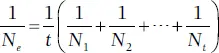
In words, the harmonic mean is the reciprocal of the average of reciprocals of the population size for each of t generations. This method of estimating an effective population gives more weight to smaller population sizes. For example, the N efor three generations (t = 3) in which N 1= 1000, N 2= 10, and N 3= 1000, would be
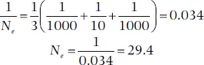
which is far less than 670, the arithmetic mean of 1000, 10, and 1000. (Also see Vucetich et al. 1997 and Lovatt and Hoelzel 2014 for the effect of population fluctuations.)
Example 2. Unequal numbers of females and males . If a population has an unbalanced sex ratio, the effective population size is less than the actual size and can be estimated as
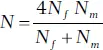
where N fis the number of breeding females and N mis the number of breeding males (Hartl and Clark 1997). For example, if 96 females mated with four males,
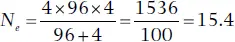
This kind of imbalance, as extreme as it may seem, is fairly common. Genetic analyses that determine the mother and father of offspring frequently indicate that in many species relatively few individuals, especially among males, are responsible for a disproportionate share of a population’s reproduction (Parker and Waite 1997). Many apparently healthy adults do not leave any offspring. Such inequity is generally not a problem – it is the basis for natural and sexual selection – but it may lead to difficulties in populations that suddenly get small because of its effect on genetic diversity. Consider the endangered Española Island giant tortoise of the Galápagos (see Case Study 1.1, “Return of the Tortoises to Española”). These tortoises likely numbered in the thousands but after most were killed for food by early mariners the population plummeted to 15, consisting of 12 females and just three males, which fortunately were rescued, placed in captivity, and have produced more than 1200 offspring since 1950 that have been released back to the island where they now breed on their own (Gibbs et al. 2014). Sounds like a success? It is. But it has also been discovered that the unequal sex ratio of those 15 survivors along with the unequal reproductive activity among them had led to a genetic effective population size of just 5.7 tortoises, far smaller than the census size of 15 might suggest (Milinkovitch et al. 2004). What little genetic variation remains in this population is severely threatened by the genetic drift exerted during the very long and “tight” bottleneck this species endured for many decades. Carefully managed pairings of surviving tortoises are now being made to maximize “capture” of what little genetic diversity remains for the newer generations. The bottom line to remember is that the effective population size is often substantially less than the actual number of individuals in a population, often only 10–20% (Vucetich et al. 1997). Thus, if you want a “population” of bison with N e= 100 (hopefully sufficient to retain 99.5% of its genetic variability through at least one generation; see Table 5.3), you actually need a census population of somewhere between 500 and 1000.
Читать дальшеИнтервал:
Закладка:
Похожие книги на «Fundamentals of Conservation Biology»
Представляем Вашему вниманию похожие книги на «Fundamentals of Conservation Biology» списком для выбора. Мы отобрали схожую по названию и смыслу литературу в надежде предоставить читателям больше вариантов отыскать новые, интересные, ещё непрочитанные произведения.


Обсуждение, отзывы о книге «Fundamentals of Conservation Biology» и просто собственные мнения читателей. Оставьте ваши комментарии, напишите, что Вы думаете о произведении, его смысле или главных героях. Укажите что конкретно понравилось, а что нет, и почему Вы так считаете.