James K. Peckol - Introduction to Fuzzy Logic

Let's look at another example. Consider that a car might be traveling on a freeway at a velocity between 20 and 90 mph. In the fuzzy world, we identify or define such a range as the universe of discourse . Within that range, we might also say that the range of 50–60 is the average velocity.

In the fuzzy context, the term average would be classed as a linguistic variable. A velocity below 50 or above 60 would not be considered a member of the average range. However, values within and equal to the two extrema would be considered members.

The following paragraphs are partially reused in Chapter 4.

The fuzzy property “close to 7” can be represented in several different ways. Who decides what that representation should be? That task falls upon the person doing the design.

To formulate a membership function for the fuzzy concept “close to 7,” one might hypothesize several desirable properties. These might include the following properties:

Normality – It is desirable that the value of the membership function (grade of membership for 7 in the set F) for 7 be equal to 1, that is, μF(7) = 1.We are working with membership values 0 or 1.

Monotonicity – The membership function should be monotonic. The closer r is to 7, the closer μF(r) should be to 1.0 and vice versa.We are working with membership values in the range 0.0–1.0.

Symmetry – The membership function should be one such that numbers equally distant to the left and right of 7 have equal membership values.We are working with membership values in the range 0.0–1.0.

It is important that one realize that these criteria are relevant only to the fuzzy property “close to 7” and that other such concepts will have appropriate criteria for designing their membership functions.

Based on the criteria given, graphic expressions of the several possible membership functions may be designed. Three possible alternatives are given in Figure 1.3. Depending upon whether one is working in a crisp or fuzzy domain, the range of grade of membership (vertical) axis should be labeled either {0–1} or {0.0–1.0}.

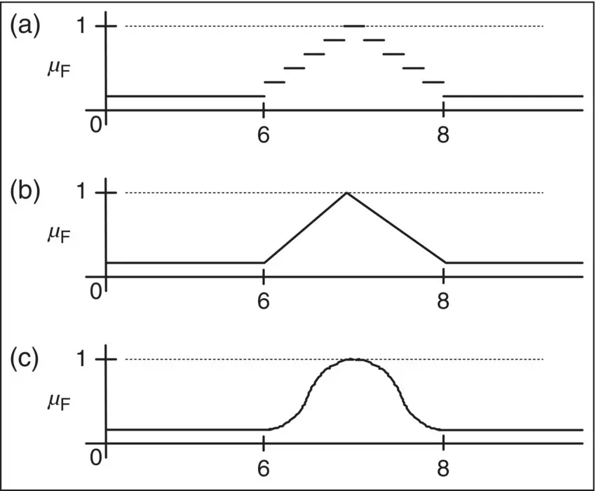
Figure 1.3 Membership functions for “close to 7.”

Note that in graph c, every real number has some degree of membership in F although the numbers far from 7 have a much smaller degree. At this point, one might ask if representing the property “close to 7” in such a way makes sense.

Consider a shopping trip with a friend in Paris who poses the question:

How much does that cost?

To which you answer:

About 7 euros.

which certainly can be represented graphically.

As a further illustration, let the crisp set H and the fuzzy subset F represent the heights of players on a basketball team. If, for an arbitrary player p , we know that the membership in the set H is given as μ H( p ) = 1, then all we know is that the player's height is somewhere between 6 and 8 ft. On the other hand, if we know that the membership in the set P is given as μ F( p ) = 0.85, we know that the player's height is close to 7 ft. Which information is more useful?

Consider the phrase:

Etienne is old.

The phrase could also be expressed as:

Etienne is a member of the set of old people.

If Etienne is 75, one could assign a fuzzy truth value of 0.8 to the statement. As a fuzzy set, this would be expressed as:

μold (Etienne) = 0.8

From what we have seen so far, membership in a fuzzy subset appears to be very much like probability. Both the degree of membership in a fuzzy subset and a probability value have the same numeric range: 0–1. Both have similar values: 0.0 indicating (complete) nonmembership for a fuzzy subset and FALSE for a probability and 1.0 indicating (complete) membership in a fuzzy subset and TRUE for a probability. What, then, is the distinction?

Consider a natural language interpretation of the results of the previous example. If a probabilistic interpretation is taken, the value 0.8 suggests that there is an 80% chance that Etienne is old. Such an interpretation supposes that Etienne is or is not old and that we have an 80% chance of knowing it. On the other hand, if a fuzzy interpretation is taken, the value of 0.8 suggests that Etienne is more or less old (or some other term corresponding to 0.8).

To further emphasize the difference between probability and fuzzy logic, let's look at the following example.

Let

L = the set of all liquids

P = the set of all potable liquids

Suppose that you have been in the desert for a week with nothing to drink, and you find two bottles ( Figure 1.4).

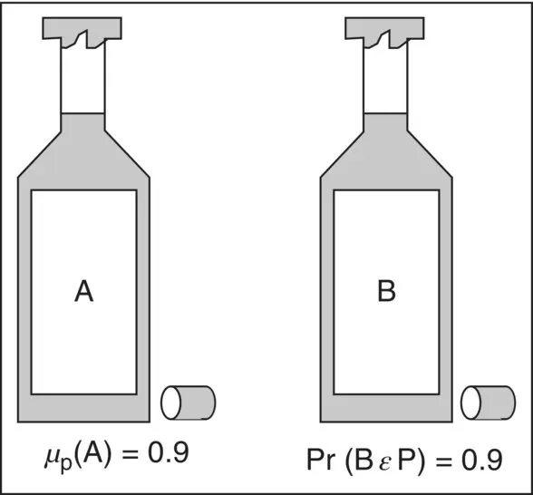
Figure 1.4 Bottles of liquids – front side.

Which bottle do you choose?

Bottle A could contain wash water. Bottle A could not contain sulfuric acid.

A membership value of 0.9 means that the contents of A are very similar to perfectly potable liquids, namely, water.

A probability of 0.9 means that over many experiments that 90% yield B to be perfectly safe and that 10% yield B to be potentially deadly. There is 1 chance in 10 that B contains a deadly liquid.

Observation:

What does the information on the back of the bottles reveal?

After examination, the membership value for A remains unchanged, whereas the probability value for B containing a potable liquid drops from 0.9 to 0.0 ( Figure 1.5).

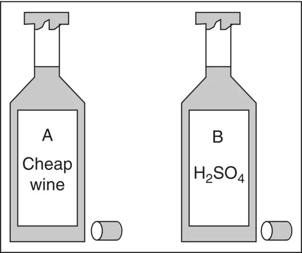
Figure 1.5 Bottles of liquids – back side.

As the previous example illustrates, fuzzy memberships represent similarities to objects that are imprecisely defined, while probabilities convey information about relative frequencies.

Expert systems are an outgrowth of postproduction systems augmented with various elements of probability theory and fuzzy logic to emulate human reasoning within constrained domains. The general structure of such systems is a decision‐making portion known as an inference engine associated with a hierarchical knowledge structure or knowledge base .

The knowledge base typically consists of the domain‐specific knowledge and at least one level of abstraction. This second level contains the knowledge about knowledge or metaknowledge for the domain. As such, this level of abstraction provides the inference engine with the criteria for making decisions or reasoning within the specific domain of application.

In some cases, these systems have performed with remarkable success. Most notables are Dendral, Feigenbaum (1969), Meta‐Dendral , Buchanan (1978), Rule‐Based Expert Systems: MYCIN Experiments, Shortliffe (1984), and Prospector, Duda (1978). In each case, there have been tens and perhaps hundreds of man‐years devoted to tailoring each to a specific task. Nonetheless, those could be integrated, with very little effort, as a brute‐force solution to reasoning. These systems have little ability to learn from previous experience and are extremely fragile at the boundaries of their knowledge.