Cory Althoff - The Self-Taught Computer Scientist

Figure 1.2shows what it looks like when you plot a logarithmic algorithm.

The required number of steps grows more slowly in a logarithmic algorithm as the data set gets larger.

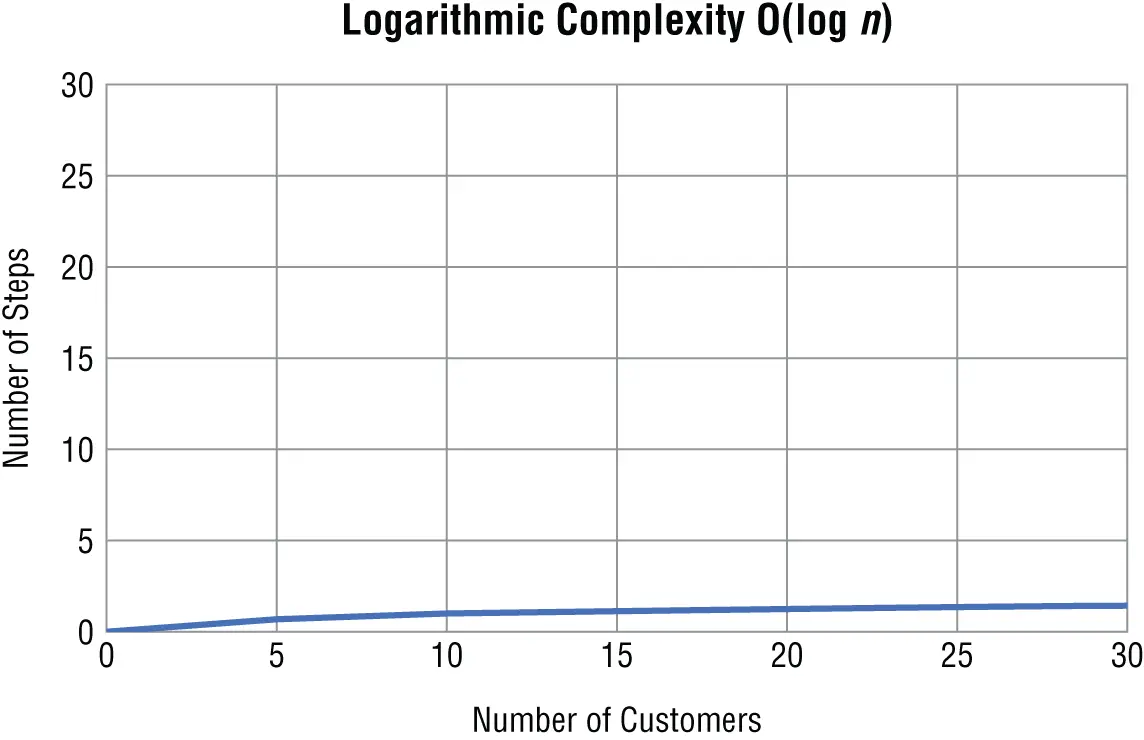
Figure 1.2Logarithmic complexity

The next most efficient type of algorithm is one that runs in linear time. An algorithm that runs in linear timegrows at the same rate as the size of the problem. You express a linear algorithm in big O notation as O( n ).

Suppose you must modify your free book program so that instead of giving a free book to the first customer of the day, you iterate through your list of customers and give them a free book if their name starts with the letter B . This time, however, your list of customers isn't sorted alphabetically. Now you are forced to iterate through your list one by one to find the names that start with B .

free_book = False customers = ["Lexi", "Britney", "Danny", "Bobbi", "Chris"] for customer in customers: if customer[0] == 'B': print(customer)

When your customer list contains five items, your program takes five steps to complete. For a list of 10 customers, your program requires 10 steps; for 20 customers, 29 steps; and so on.

This is the equation for the time complexity of this program:

f(n) = 1 + 1 + n

And in big O notation, you can ignore the constants and focus on the part that dominates the equation:

O(n) = n

In a linear algorithm, as n gets bigger, the number of steps your algorithm takes increases by however much n increases ( Figure 1.3).

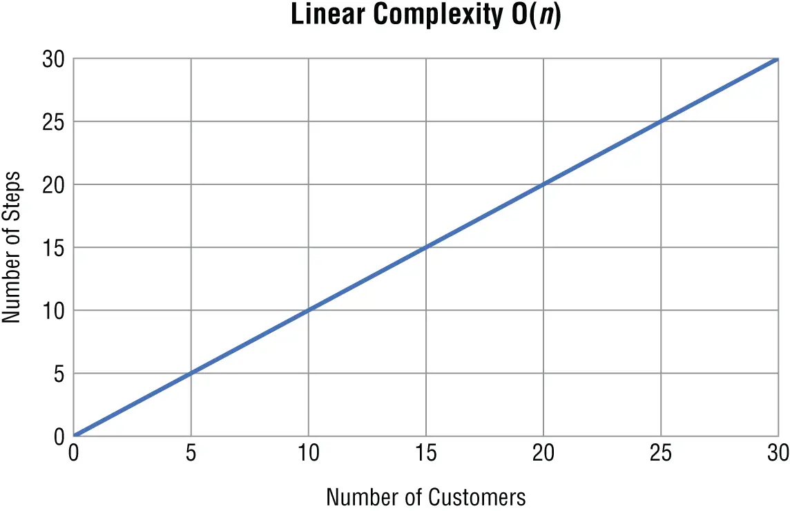
Figure 1.3Linear complexity

An algorithm that runs in log-linear timegrows as a combination (multiplication) of logarithmic and linear time complexities. For example, a log-linear algorithm might evaluate an O(log n ) operation n times. In big O notation, you express a log-linear algorithm as O( n log n ). Log-linear algorithms often divide a data set into smaller parts and process each piece independently. For example, many of the more efficient sorting algorithms you will learn about later, such as merge sort, are log-linear.

Figure 1.4shows what a log-linear algorithm looks like when you plot it on a graph.

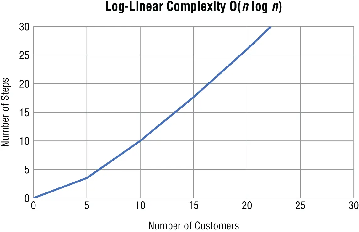
Figure 1.4Log-linear complexity

As you can see, log-linear complexity is not as efficient as linear time. However, its complexity does not grow nearly as quickly as quadratic, which you will learn about next.

After log-linear, the next most efficient time complexity is quadratic time. An algorithm runs in quadratic timewhen its performance is directly proportional to the problem's size squared. In big O notation, you express a quadratic algorithm as O( n **2).

Here is an example of an algorithm with quadratic complexity:

numbers = [1, 2, 3, 4, 5] for i in numbers: for j in numbers: x = i * j print(x)

This algorithm multiplies every number in a list of numbers by every other number, stores the result in a variable, and prints it.

In this case, n is the size of your numberslist. The equation for this algorithm's time complexity is as follows:

f(n) = 1 + n * n * (1 + 1)

The (1 + 1) in the equation comes from the multiplication and print statement. You repeat the multiplication and print statement n * n times with your two nested forloops. You can simplify the equation to this:

f(n) = 1 + (1 + 1) * n**2

which is the same as the following:

f(n) = 1 + 2 * n**2

As you may have guessed, the n **2 part of the equation overshadows the rest, so in big O notation, the equation is as follows:

O(n) = n**2

When you graph an algorithm with quadratic complexity, the number of steps increases sharply as the problem's size increases ( Figure 1.5).

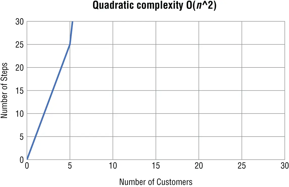
Figure 1.5Quadratic complexity

As a general rule, if your algorithm contains two nested loops running from 1 to n (or from 0 to n − 1), its time complexity will be at least O( n **2). Many sorting algorithms such as insertion and bubble sort (which you will learn about later in the book) follow quadratic time.

After quadratic comes cubic time complexity. An algorithm runs in cubic timewhen its performance is directly proportional to the problem's size cubed. In big O notation, you express a cubic algorithm as O( n **3). An algorithm with a cubic complexity is similar to quadratic, except n is raised to the third power instead of the second.

Here is an algorithm with cubic time complexity:

numbers = [1, 2, 3, 4, 5] for i in numbers: for j in numbers: for h in numbers: x = i + j + h print(x)

The equation for this algorithm is as follows:

f(n) = 1 + n * n * n * (1 + 1)

Or as follows:

f(n) = 1 + 2 * n**3

Like an algorithm with quadratic complexity, the most critical part of this equation is n **3, which grows so quickly it makes the rest of the equation, even if it included n **2, irrelevant. So, in big O notation, quadratic complexity is as follows:

O(n) = n**3

While two nested loops are a sign of quadratic time complexity, having three nested loops running from 0 to n means that the algorithm will follow cubic time. You will most likely encounter cubic time complexity if your work involves data science or statistics.

Both quadratic and cubic time complexities are special cases of a larger family of polynomial time complexities. An algorithm that runs in polynomial timescales as O( n ** a ), where a = 2 for quadratic time and a = 3 for cubic time. When designing your algorithms, you generally want to avoid polynomial scaling when possible because the algorithms can get very slow as n gets larger. Sometimes you can't escape polynomial scaling, but you can find comfort knowing that the polynomial complexity is still not the worst case, by far.

The honor of the worst time complexity goes to exponential time complexity. An algorithm that runs in exponential timecontains a constant raised to the size of the problem. In other words, an algorithm with exponential time complexity takes c raised to the n th power steps to complete. The big O notation for exponential complexity is O( c ** n ), where c is a constant. The value of the constant doesn't matter. What matters is that n is in the exponent.

Fortunately, you won't encounter exponential complexity often. One example of exponential complexity involving trying to guess a numerical password consisting of n decimal digits by testing every possible combination is O(10** n ).

Here is an example of password guessing with O(10** n ) complexity: