William Puech - Multimedia Security, Volume 1

Our objective is to recognize each step of the production chain of an image. This information can sometimes appear in the data accompanying the image, called EXIF (Exchangeable Image File Format), which also includes information such as the brand and model of the camera and lens, the time and location of the photograph, and its shooting settings. However, this information can be easily modified, and is often automatically deleted by social media for privacy reasons. Therefore, we are interested in the information left by the operations on the image itself rather than in the metadata. Some methods, like the one presented in Huh et al . (2018), offer to check the consistency of the data present in the image with its EXIF metadata.

Knowledge of the image production chain allows for the detection of changes.

A first application is the authentication of the camera model. The processing chain is specific to each device model; so it is possible to determine the device model by identifying the processing chain, as implemented in Gloe (2012) where features are used to classify photographs according to their source device. More recently, Agarwal and Farid (2017) showed that even steps common to many devices, such as JPEG compression, sometimes have implementation differences that allow us to differentiate models from multiple manufacturers, or even models from the same manufacturer.

Another application is the detection of suspicious regions in an image, based on the study of the residue – sometimes called noise – left by the processing chain. This residue is constituted of all the traces left by each operation. While it is often difficult, or even impossible, to distinguish each step in the processing chain individually, it is easier to distinguish two different processing chains as a whole. Using this idea, Cozzolino and Verdoliva proposed to use steganography tools (see Chapter 5entitled “Steganography: Embedding data into Multimedia Content”) to extract the image residue (Cozzolino et al . 2015b). Treating this residue as a piece of hidden information in the image, an algorithm such as Expectation–Maximization (EM) is then used to classify the different regions of the image. Subsequently, neural networks have shown good performance in extracting the residue automatically (Cozzolino and Verdoliva 2020; Ghosh et al . 2019), or even in carrying out the classification themselves (Zhou et al . 2018).

The outline of this chapter arises from previous considerations. Section 1.2describes the main operations of the image processing chain.

Section 1.3is dedicated to the effect each step of the image processing pipeline has on the image’s noise. This section illustrates how and why the fine analysis of noise enables the reverse engineering of the image and leads to the detection of falsified areas because of the discrepancies in the noise model.

We then detail the two main operations that lead to the final coding of the image. Section 1.4explains how demosaicing traces can be detected and analyzed to detect suspicious areas of an image. Section 1.5describes JPEG encoding, which is usually the last step in image formation, and the one that leaves the most traces. Similarly to demosaicing, we show how the JPEG encoding of an image can be reverse-engineered to understand its parameters and detect anomalies. The most typical cases are cropping and local manipulations, such as internal or external copy and paste.

Section 1.6specifically addresses the detection of internal copy-move, a common type of manipulation. Finally, section 1.7discusses neural-network-based methods, often efficient but at the cost of interpretability.

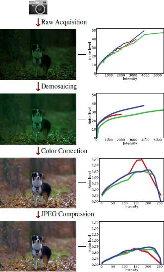
Figure 1.2. Simplified processing pipeline of an image, from its acquisition by the camera sensor to its storage as a JPEG-compressed image. The left column represents the image as it goes through each step. The right column plots the noise of the image as a function of intensity in all three channels (red, green, blue). Because each step leaves a specific footprint on the noise pattern of the image, analyzing this noise enables us to reverse engineer the pipeline of an image. This in turn enables us to detect regions of an image which were processed differently, and are thus likely to be falsified

The main steps in the digital image acquisition process, illustrated in Figure 1.2, will be briefly described in this section. Other very important steps, such as denoising, are beyond the scope of this chapter and will therefore not be covered here.

The first step of acquiring a raw image consists of counting the number of incident photons over the sensor along the exposure time. There are two different technologies used in camera sensors: charge coupled devices (CCDs) and complementary metal-oxide-semiconductors (CMOS). Although their operating principles differ, both can be modeled in a very similar way (Aguerrebere et al . 2013). Both sensors transform incoming light photons into electronic charge, which interacts with detection devices to produce electrons stored in a potential light well. When the latter is full, the pixels become saturated. The final step is to convert the analog voltage measurements into digital quantized values.

Most cameras cannot see color directly, because each pixel is obtained through a single sensor that can only count the number of photons reaching it in a certain wavelength range. In order to obtain a color image, a color filter array (CFA) is placed in front of the sensors. Each of them only counts the photons of a certain wavelength. As a result, each pixel has a value relative to one color. By using filters of different colors on neighboring pixels, the missing colors can then be interpolated.

Although others exist, almost all cameras use the same CFA: the Bayer array, which is illustrated in Figure 1.3. This matrix samples half the pixels in green, a quarter in red and the last quarter in blue. Sampling more pixels in green is justified by the human visual system, which is more sensitive to the color green.

Unlike other steps in the formation of an image, a wide variety of algorithms are used to demosaic an image. The most simple demosaicing algorithm is bilinear interpolation: missing values are interpolated by averaging the most direct neighbors sampled in that channel. As the averaging is done regardless of the image gradient, this can cause visible artifacts when interpolated against a strong gradient, such as on image edges.

To avoid these artifacts, more recent methods attempt to simultaneously take into account information from the three color channels and avoid interpolation along a steep gradient. For instance, the Hamilton–Adams method is carried out in three stages (Hamilton and Adams 1997). First, it interpolates the missing green values by taking into account the green gradients corrected for the discrete Laplacian of the color already known at each pixel to interpolate horizontally or vertically, in the direction where the gradient is weakest. It then interpolates the red and blue channels on the pixels sampled in green, taking the average of the two neighboring pixels of the same color, corrected by the discrete Laplacian of the green channel in the same direction. Finally, it interpolates the red channel of blue-sampled pixels and the blue channel of red-sampled pixels using the corrected average of the Laplacian of the green channel, in the smoothest diagonal.